Original Feishu document · Source revision 27

💡

Course positioning: This chapter belongs to the “value, reward, and learning from experience” track. RECAP serves as a case study; the main objective is to understand what supervision is provided by rewards, returns, values, advantages, human corrections, and offline data, and how these signals connect to VLAs, world models, and the data flywheel.

1. What Signals Can Make a Robot Change Its Behavior

Learning objectives: After completing this chapter, you should be able to distinguish among demonstrated actions, success labels, stepwise rewards, preference comparisons, value estimates, and human corrections; interpret returns, values, and advantages; understand the critic through the Bellman recursion; derive KL-regularized policy improvement; and design ablations that distinguish “more data” from “better learning algorithms.”

Supervision signal	What it directly tells the model	Typical objective	What it does not directly tell the model
Expert actions	What the expert did in this state	Behavior cloning	Why other actions are worse
Task-success labels	Whether the entire trajectory completed the task	Return and value learning	Which specific step caused the outcome
Stepwise rewards	Local quality at each stage	Reinforcement learning	Safety constraints and preferences not encoded by the reward
Pairwise preferences	Whether trajectory A is better than trajectory B	Reward modeling and preference optimization	An absolute value scale
Human corrections	How to recover from an erroneous state	Corrective imitation and DAgger-style methods	How to rank actions in regions without intervention
Failure data	Which undesirable states the policy actually enters	Value learning, classifiers, and data reweighting	The correct action in a failure state, unless a correction is also provided

These signals can be combined. The key idea behind RECAP is not simply to “train on failures,” but to organize autonomous execution, task outcomes, value estimation, and human recovery demonstrations into a policy-improvement loop.

2. From Reward to Value: How to Read the Bellman Recursion

After taking action in state , the agent receives reward . The discounted return beginning at time is:

Interpretation: The return from the current time equals the sum of the current and future rewards, each multiplied by a discount factor according to how many steps it lies in the future.

Derivation: This is the definition of the finite-horizon discounted return. A smaller gamma places more emphasis on near-term outcomes; when gamma equals one, the rewards are accumulated without discounting.

Read this as: “Starting from the current time, add future rewards after discounting them according to how far away they are.” The state value and action value are defined respectively as:

Interpretation: The state value is the conditional expectation of the future return when the current state is s and the agent subsequently follows policy pi.

Derivation: Even from the same state, policy sampling and environmental stochasticity may produce multiple trajectories. The state value averages the returns of those trajectories.

Interpretation: The action value is the conditional expectation of the future return when action a is first taken in state s and policy pi is followed thereafter.

Derivation: Further conditioning the expected cumulative return G_t on the current action a yields the state-action value Q. Compared with V, it additionally captures the long-term consequences of first taking action a in state s.

Q fixes the current action in addition to the current state, so it can be used to compare the long-term outcomes of different actions in the same state.

These are not labels that have already been observed; they are conditional expectations over stochastic future outcomes. The Bellman equation decomposes the long-horizon return into the one-step reward and the value of the next state:

Interpretation: The value of the current state-action pair equals the current one-step reward plus the discounted value of the next state, with a conditional expectation taken over the environment transition.

Derivation: Decompose the return G_t into the current reward r_t plus gamma times the return at the next time step. The conditional expectation of that next return is V.

The advantage measures how much better an action is than the current policy’s average:

Interpretation: The advantage of action a in state s equals its action value minus the average value of the current policy in that state.

Derivation: V is the average of Q under the current policy’s action distribution, so subtracting it gives the incremental value of an action relative to the average choice.

Read this as: “How much better is taking action in state than the average choice under the current policy?” A positive advantage means the action’s probability should be increased, while a negative advantage means it should be decreased.

2.1 Why Value Functions Can Be Wrong

A critic can estimate values reliably only near the states and actions covered by the data. For actions absent from the offline dataset, the value network may assign spuriously high scores because of function extrapolation. Contact-rich tasks also present a severe credit-assignment problem: an eventual failure may have been caused by a slight slip much earlier rather than by the final action.

2.2 The Relationship Between Value Learning and World Models

A value function directly compresses future returns without having to predict future states. A world model predicts the future following an action, after which a reward or value function evaluates whether that future is desirable. The two can be combined: the world model generates imagined rollouts, and the value function evaluates their endpoints. They can also remain entirely separate, as model-free RL directly learns the value function and policy.

3. π0.6* and RECAP: A Case Study in Improving Large-Model Policies

π0.6 is a further engineered version of π0.5, featuring a larger Gemma 3 4B backbone, an Action Expert with approximately 860M parameters, richer conditioning inputs, and Knowledge Insulation to protect the VLM’s general-purpose knowledge from degradation by robot-action objectives.

The key idea behind Knowledge Insulation is that discrete-action and semantic supervision can train the shared backbone, while gradients from the continuous Flow Matching expert are prevented from flowing backward into and contaminating the VLM Backbone. It does not freeze the backbone completely; instead, it controls the gradient paths of different losses.

4. Why Imitation Learning Accumulates Errors

After the policy makes a small error, the environment enters a state that is sparsely represented in the expert data. Continuing to use the original policy causes the deviation to grow. The solution is not merely to add more perfect demonstrations, but to collect the failure states that the model actually encounters.

5. RECAP’s Data Loop

1. Execute tasks on real robots using the current policy.
2. Collect autonomous successes, failures, and trajectories corrected through human intervention.
3. Train the value function V(o,l) from task outcomes.
4. Estimate the advantage A(o,a,l) of each action relative to the value of the current state.
5. Convert the advantage into a conditioning input and train the policy to prefer high-advantage actions.
6. Deploy the new policy and begin the next round of data collection.

6. Deriving Advantage Conditioning from KL-Regularized Policy Improvement

Consider maximizing advantage while constraining the policy from deviating too far from the reference policy π_ref:

Interpretation: For a fixed observation o, find a policy that maximizes the expected advantage under the reference policy while penalizing deviation from that reference policy using a KL divergence weighted by beta.

Derivation: The first term encourages the new policy to select actions with high advantage under the reference policy. The second term uses KL divergence to penalize deviation from the reference policy. Beta controls the trade-off between the magnitude of improvement and stability.

Motivation for the derivation: The first term pushes the policy toward high-advantage actions, while the second limits the update magnitude, preventing critic errors from causing a large policy to move too far outside the data distribution in a single update.

For ease of interpretation, first consider discrete actions. Fix observation o and add the constraint that the action probabilities sum to one:

Interpretation: The Lagrangian consists of three parts: expected advantage, a negative KL penalty, and a policy-probability normalization constraint.

Derivation: Expand the expected advantage as a weighted sum over discrete actions, expand the definition of the KL divergence, and use the Lagrange multiplier lambda to impose the constraint that the probabilities of all actions sum to 1. This yields the stated objective.

Take the partial derivative with respect to each action probability and set it to zero:

Interpretation: At the optimum, the action advantage, the logarithmic ratio of the policy to the reference policy, and the normalization multiplier must be in equilibrium.

Derivation: Differentiate the Lagrangian with respect to each pi(a|o): the advantage term contributes A, the KL term contributes negative beta times the log ratio plus 1, and the normalization constraint contributes lambda. Setting the derivative to zero yields the stationarity condition.

Rearrange and exponentiate. All action-independent terms are absorbed into the normalization constant. For continuous actions, replace the sum with an integral; the conclusion remains the same.

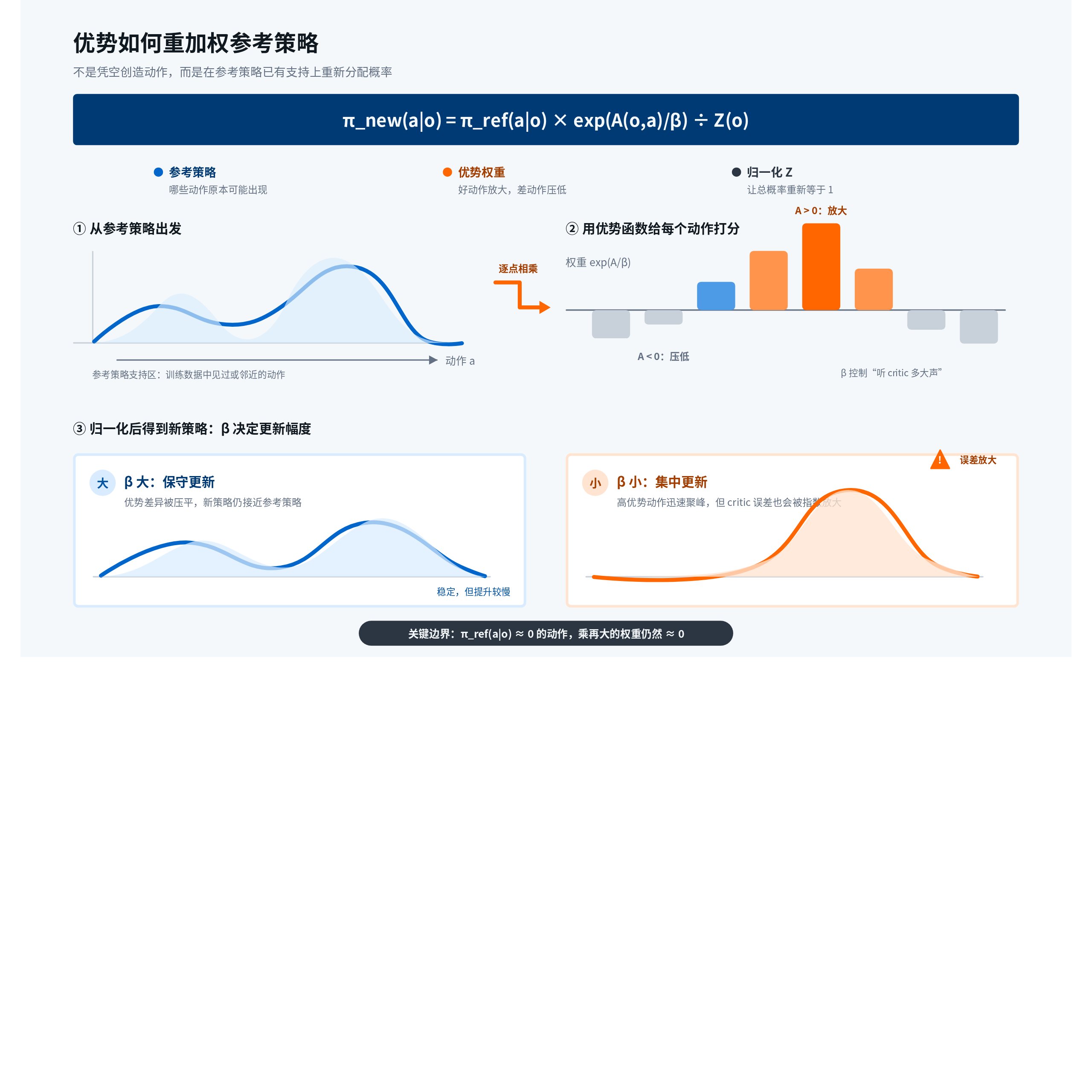
Interpretation: The new policy equals the reference policy multiplied by an exponential advantage weight and then divided by the observation-dependent normalization constant Z.

Derivation: The preceding equation gives the proportional relationship. Summing or integrating over all actions and requiring the total probability to equal one yields the denominator Z. The smaller beta is, the more concentrated the policy becomes on high-advantage actions—and the more likely it is to amplify critic errors.

Rather than applying PPO directly to a large Flow VLA, RECAP binarizes the advantage into an improvement indicator I and trains a conditional policy π(a|o,I). At inference time, the policy is always conditioned to request high-advantage actions.

Formula Visualization｜How Advantage Reweights the Reference Policy

7. Division of Labor Between Human Corrections and Reinforcement Learning

Signal	Best suited to solving	Limitations
Human intervention and correction	Teaching the model how to recover from specific erroneous states	Expensive and requires real-time expert participation
Task rewards and autonomous trials	Distinguishing good behavior from bad behavior at scale and improving success rate and throughput	Rewards are sparse, and value estimates may be biased

8. Experimental Issues That Require Caution

• Success-rate improvements may come from the additional data rather than from advantage conditioning itself; comparison against an equal amount of SFT data is required.
• Value-function errors may attribute accidental successes to the wrong actions; calibration across initial states and task stages is required.
• Higher throughput may compromise action safety margins; collisions, peak forces, and human-intervention rates should be reported separately.

9. How This Approach Connects VLAs, World Models, and Data Engines

Connection	Mechanism	Primary risk
Value → VLA	Weight, condition, or rerank actions to increase the probability of high-advantage actions	Critic bias is amplified by the policy
World model → value	Use imagined rollouts to generate future-return training signals	Model errors contaminate the value estimates
VLA → data engine	Deploy the current policy and collect autonomous successes, failures, and human interventions	Online exploration and safety costs
Data engine → value	Provide success labels, stage outcomes, and the failure distribution	Label delays and inconsistent task definitions
Human corrections → policy	Directly provide recovery actions in erroneous states	The intervention policy introduces selection bias

Decisive Experiments

1. Equal-data control: Fix the number of newly added trajectories and compare standard SFT, success filtering, advantage weighting, and conditional policies.
2. Value calibration: Bin examples by predicted value, compare their actual success rates, and report ECE or reliability curves.
3. Task-stage stratification: Evaluate the approach, contact, manipulation, release, and recovery stages separately rather than reporting only whole-task success rates.
4. Safety metrics: Report collisions, peak forces, human-intervention rates, and recovery times together.
5. Out-of-distribution validation: Test whether value rankings remain consistent across novel objects, initial states, and dynamics parameters.

Improvements can be attributed to the experience-learning mechanism rather than simple growth in dataset size only when equal-data controls still show policy improvement, value predictions are calibrated against actual outcomes, and safety metrics do not degrade.

Exercises

1. Derive the closed-form solution for the exponentially weighted policy using Lagrange multipliers.
2. Design an ablation experiment that distinguishes the benefit of correction data from the benefit of RL.
3. Explain why failure trajectories should not simply be deleted, and why their state, recovery, and outcome information should instead be retained.

Primary Sources