Original Feishu Document · Source Revision 28

💡

Mechanisms Lesson: Building on B0, this lesson addresses one specific question: How can high-dimensional, partially observable robot observations be compressed into latent states that can predict the future, rewards, and termination? The focus is on probabilistic graphical models, state-space models, filtering, the ELBO, and multi-step rollouts.

Learning Objectives and Prerequisites

Prerequisites include conditional probability, expectation, variance, and KL divergence. After completing this lesson, you should be able to distinguish among true states, observations, belief states, and latent states; write the joint distribution of a state-space model; derive the variational lower bound; explain why accurate one-step prediction does not necessarily yield usable long-horizon rollouts; and design representation ablations oriented toward prediction and control.

1. States, Observations, and Beliefs

A partially observable system can be written as:

Read as: Given the current true state s_t and action a_t, the next true state s_{t+1} is sampled from the environment's transition distribution.

Derivation: This is the definition of controlled Markov dynamics. If the current state already contains the information needed to predict the future, then the earlier history becomes conditionally independent given s_t and a_t and can be eliminated.

Read as: The current observation o_t is generated stochastically from the current true state s_t through the observation model.

Derivation: Sensors observe only the result of imaging, noise, and occlusion applied to the true state. The observation is therefore a conditional random variable of the state and need not equal the state itself.

The policy can observe only and therefore requires a belief distribution:

Read as: The probability assigned by belief b_t to state value s equals the posterior probability that the current true state is s, conditioned on all observations up to the present and all preceding actions.

Derivation: Under partial observability, a single observation frame cannot be treated directly as the state. Conditioning the unobserved state on all available history yields the posterior distribution used for decision-making.

This is read as: “The posterior distribution of the current true state, conditioned on all historical observations and past actions.” When a robot cannot directly observe friction, occluded objects, or contact forces, a belief is more faithful than a point estimate.

1.1 Bayesian Filtering

Prediction step:

Read as: The predicted belief is obtained by integrating over all states at the previous time step: the belief weight of each previous state is multiplied by the probability of transitioning from that state to the current state under the action.

Derivation: By the law of total probability, the unknown s_{t-1} is marginalized out; the Markov assumption reduces the transition term to p(s_t|s_{t-1},a_{t-1}).

Update step:

Read as: The updated belief equals the observation likelihood multiplied by the predicted belief, divided by a normalization constant obtained by summing or integrating over all candidate states.

Derivation: This follows directly from Bayes' rule. The numerator increases the weights of states that explain the new observation, while the denominator p(o_t|history) ensures that the updated belief integrates to 1.

The first step propagates the dynamics to the current time, and the second corrects the result using the new observation. Deep models typically approximate this process using an RNN, Transformer, or stochastic latent variables.

2. State-Space Models

A latent state-space model consists of representation, transition, and observation-generation components:

Read as: Based on the observation history and preceding actions, the inference model q_psi produces an approximate posterior distribution over the current latent state z_t.

Derivation: The true posterior is generally not analytically tractable, so a trainable encoder is used to approximate Bayesian filtering. A sampling-based formulation can also represent the possibility that the same observation history corresponds to multiple hidden states.

Read as: Based on the current latent state and action, the latent dynamics produce a conditional distribution over the next latent state.

Derivation: This model projects the true controlled state transition into latent space. If z_t is sufficient for prediction, it can compress the earlier history.

Read as: Based on latent state z_t, the observation decoder generates a conditional distribution over the current observation o_t.

Derivation: A generative model must specify how latent variables explain visible data. Choosing a Gaussian distribution, a discrete pixel distribution, or a perceptual feature distribution leads to different reconstruction losses.

Joint distribution:

Read as: Given the first T-1 actions, the joint probability of the complete observation and latent-state sequences is obtained by multiplying the initial-state term, T observation-generation terms, and T-1 action-conditioned transition terms.

Derivation: First expand the joint distribution using the chain rule, then remove redundant conditions using the Markov conditional-independence assumption for state transitions and the assumption that each observation depends only on the current latent state. The transition product must end at T-1; otherwise, z_{T+1} would be introduced incorrectly.

3. ELBO: Why Both Reconstruction and Prediction Matter

The log-likelihood of the observation sequence is:

Read as: This is the log marginal likelihood that the model assigns to the entire observation sequence given the action sequence.

Derivation: It is obtained by marginalizing the joint distribution over all latent trajectories. This high-dimensional integral is usually intractable, so a variational lower bound is required.

Introduce the approximate posterior :

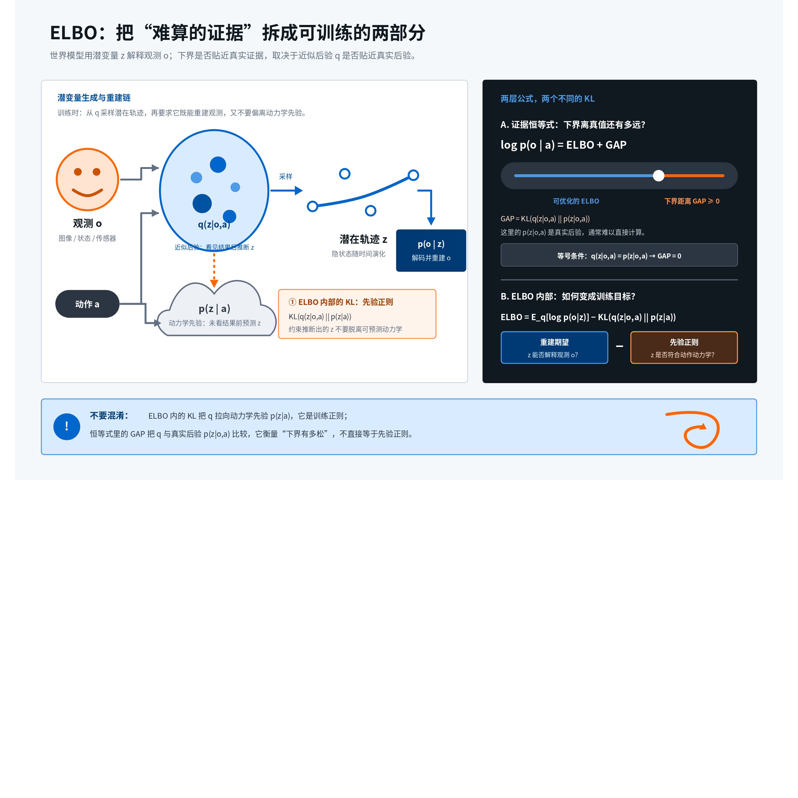
Read as: The observation log-likelihood equals the evidence lower bound plus the KL divergence between the approximate posterior and the true posterior.

Derivation: Multiply and divide by q(z|o,a) inside log p(o|a), take the expectation under q, and rearrange the terms. The remaining difference is exactly the KL divergence. Here, o, z, and a denote their respective complete sequences.

Because KL divergence is nonnegative:

Read as: The observation log-likelihood is no smaller than the evidence lower bound.

Derivation: The KL divergence in the preceding identity is always nonnegative, so removing it yields a lower bound that cannot exceed the true log-likelihood. Equality holds when the approximate posterior equals the true posterior.

A common form is:

Read as: The ELBO equals the expected observation-reconstruction log-probability under the approximate posterior, minus the KL divergence between the complete posterior trajectory and the action-conditioned dynamics prior.

Derivation: Factor the joint distribution into the observation-generation terms and the latent-trajectory prior, then regroup the expectation of log p(o,z|a)-log q(z|o,a). This yields the reconstruction term minus the KL term.

The first term measures the ability to explain observations, while the second measures consistency between the posterior and the dynamics prior. If only reconstruction is optimized, the latent state may memorize background textures; if only prediction is optimized, the state may discard details required by the current task.

Formula Visualization｜The ELBO's Reconstruction Term, Dynamics Prior, and Posterior Gap

4. Decision-Oriented Latent States

A world model does not necessarily need to reconstruct every pixel. More importantly, the latent state should retain:

• Object poses, velocities, and contact phases.
• Hidden factors related to action outcomes.
• Information predictive of rewards and termination.
• Uncertainty and multiple possible futures.

Auxiliary objectives can be added:

Read as: The total training loss is a weighted sum of four terms: reconstruction, reward prediction, termination prediction, and contrastive learning.

Derivation: This is not a probabilistic identity but a multitask optimization objective. The lambda coefficients map tasks with different units and gradient scales into a shared objective. Some weights can be interpreted as noise variances only when an explicit joint-likelihood assumption is specified.

More auxiliary tasks are not necessarily better. Each objective may alter the representation's inductive bias and should be validated through control performance rather than prediction metrics alone.

5. Multi-Step Rollouts and Error Accumulation

One-step prediction error:

Read as: The one-step latent error is the Euclidean distance between the next true latent state and the latent state predicted by the model.

Derivation: This defines error under a chosen latent coordinate system and L2 norm. Because latent space can be scaled or rotated, comparisons across models should either use a fixed encoder or employ decodable task metrics instead of comparing this value alone.

The model's own prediction becomes the input at the next step:

Read as: The prediction at step k+1 is obtained by having the model propagate its own step-k prediction forward again using the corresponding action.

Derivation: After the first step, an open-loop rollout no longer receives the true latent state. Consequently, the input distribution at every step is affected by preceding errors, producing compounding error rather than a simple sum of independent errors.

Multi-step error is therefore not merely the sum of one-step errors; the rollout may also enter latent regions that the model has never encountered. Scheduled sampling, short-horizon rollout losses, or uncertainty penalties can be used during training, but each method introduces bias and computational cost.

Evaluation	Question Answered
One-step prediction	Are the local dynamics correct?
Multi-step open-loop	Does the model's own rollout drift?
Closed-loop prediction	Can new observations correct errors?
Reward prediction	Does the model preserve task-relevant state?
Planning performance	Do predictions improve action selection?

6. Stochasticity and Uncertainty

There are two types of model uncertainty:

• Aleatoric: The physical process itself is stochastic, as in sliding direction and compliant deformation.
• Epistemic: The training data are insufficient, so the model does not know what it does not know.

The model can predict a heteroscedastic Gaussian:

Read as: Given the current latent state and action, the next latent state follows a Gaussian distribution whose mean and covariance are both predicted by the network.

Derivation: Under maximum-likelihood estimation, the negative log-likelihood of this distribution contains a residual term weighted by the inverse covariance and a log det Sigma term. The former penalizes prediction error, while the latter prevents the model from evading error by increasing its variance without bound.

Highly uncertain trajectories can be penalized during planning, but excessive conservatism may reject valuable exploration. Confidence calibration must be evaluated using simulated or real-world data.

7. Three Types of World-Model Objectives

Type	Objective	Advantage	Risk
Pixel world model	Generate realistic future observations	Strong visualization and broad data utilization	Capacity is consumed by the background
Latent dynamics	Predict control-relevant states	Efficient planning	Representation is difficult to interpret
Decision model	Predict rewards, values, policies, and termination	Directly supports decision-making	May discard information unrelated to the predefined objectives

8. Failure Modes and Diagnostics

Failure Mode	Observable Symptom	Diagnostic Experiment	Mitigation
Posterior collapse	The decoder ignores the latent variable, and KL approaches zero	Reconstruction changes little when z is masked	Restrict the decoder, use KL balancing or free bits
Representation dominated by the background	Reconstruction is sharp, but reward and contact predictions are poor	Background replacement and object-state probes	Object-centric representations, task-specific auxiliary objectives, and data augmentation
Multi-step drift	One-step error is small, but long rollouts deteriorate rapidly	Report open-loop error by horizon	Multi-step training, closed-loop replanning, and uncertainty constraints
Model ignores actions	Changing the action has almost no effect on the predicted future	Hold the state fixed and intervene on the action	Action alignment, counterfactual data, and control-relevant losses
Miscalibrated uncertainty	High-confidence trajectories fail on the real system	Reliability curves and coverage tests	Ensembles, calibration, and conservative planning
Incomparable latent coordinates	Latent MSE is low, but control does not improve	Evaluate using a fixed decoding task and the same planner	Use task metrics and closed-loop performance as the primary evidence

9. Minimal Experiment

In a one-dimensional cart system with friction, compare three representations: the true state, an image-reconstruction latent, and a reward-prediction latent.

1. Train a one-step dynamics model.
2. Measure one-step and 20-step rollouts separately.
3. Use the same CEM planner to compare target-reaching success rates.
4. Introduce changes in the friction parameter to test uncertainty calibration.
5. Report reconstruction error, reward error, planning success rate, and confidence intervals.

10. Exercises

1. Give plain-language readings of the prediction and update steps in Bayesian filtering.
2. Derive the ELBO and explain the direction of the KL term.
3. Design a counterexample with excellent background reconstruction but poor control performance.
4. Compare the sources of error in open-loop and closed-loop rollouts.
5. Define the world-model state and uncertainty for a contact task.
6. Explain why MuZero-style models do not need to generate realistic video.

11. Paper Landscape and Boundaries of Evidence

The following table distinguishes facts explicitly implemented in each paper, the authors' interpretations of the results, and the conclusions drawn in this course. Because the papers differ in observation space, action space, dataset scale, and evaluation tasks, they cannot be ranked across the board using a single score.

Work	Facts from the Paper	Authors' Interpretation	Course Assessment
PlaNet / RSSM	Learns deterministic memory and stochastic states in latent space and performs planning within the model	A compact latent can support pixel-based control	Establishes the state interface for modern latent world models, but extrapolation to contact and real robots still requires separate validation
Dreamer series	Trains the value function and actor on learned latent rollouts	Imagination-based training can reduce the need for real-world interaction	Performance depends on the joint accuracy of the dynamics, rewards, and continuation probabilities; reconstruction quality alone is insufficient
MuZero	The latent model predicts rewards, values, and policies without reconstructing observations	A model sufficient for decision-making need not realistically simulate pixels	Supports prioritizing control sufficiency, but when task objectives change, the model may lack information that was not supervised by the original objective
TD-MPC2	Jointly learns latent dynamics, value, and a policy prior, while executing short-horizon planning online	Scalable latent planning can support multitask continuous control	A strong model-based baseline; deployment on real robots must still report latency, contact behavior, and model-exploitation bias