Original Feishu document · Source revision 17

💡

Paper Lab: Rather than summarizing papers one by one, this lesson interrogates different approaches using the same task: What does each approach allow the model to learn? Which stability properties are guaranteed by structure? Which capabilities come from data? When failure occurs, should the policy, controller, model, or system be modified?

Learning Objectives

After completing this lesson, you should be able to compare MPC, impedance control, Residual RL, Domain Randomization, and online adaptation; reconstruct key objective functions; design ablations with equal compute, data, and safety budgets; and place control metrics and task success rates within the same chain of evidence.

1. Unified Experimental Task: Insertion with Clearance and Friction Uncertainty

The task consists of five phases: approach, initial contact, search and alignment, insertion, and withdrawal. Observations include vision, proprioception, and wrist force sensing. Actions may take the form of end-effector increments, desired forces, impedance parameters, or residual torques. Evaluation records success rate, completion time, peak force, impact energy, number of recoveries, and human interventions.

2. What Do the Five Types of Systems Actually Learn?

System	Primary Learning Target	Structural Prior
Trajectory optimization/MPC	Dynamics or cost models; the policy need not be learned	Online receding-horizon optimization and constraints
Impedance control	Usually no learning; mechanical relationships are manually specified	Feedback and compliance structure
Residual RL	Corrections applied on top of a baseline controller	Classical control provides the primary behavior
Domain Randomization	A policy robust over a parameter distribution	Simulator and randomization support set
Online adaptation	Dynamics context and a conditioned policy	Short histories contain identifiable information

3. MPC: Repeatedly Asking “What Happens Next?” Inside the Model

Finite-horizon optimization:

Interpretation: Subject to the predicted dynamics, the safe state set, and the safe action set, select a control sequence over the next H steps that minimizes the sum of stage costs and the terminal cost.

Derivation: Roll the dynamics forward from the current state. Each candidate control sequence generates a candidate state trajectory. Summing the error, control cost, contact risk, and terminal objective at every step yields the finite-horizon optimization problem. At each control cycle, only the first action is executed, and the problem is solved again using the new observation. Feedback can therefore continually correct model error, but the solve time must remain shorter than the replanning period.

MPC may use a hand-crafted model, or it may learn the dynamics, cost, or terminal value. Its structural capabilities come from explicit prediction, comparison among candidates, and constraint handling. If the model represents contact modes incorrectly, online replanning can mitigate but not eliminate the resulting systematic bias.

4. Residual RL: Let Learning Fill Only the Model Gaps

Combined control law:

Interpretation: The total control command equals the baseline controller command plus a learned residual, with the residual magnitude constrained to lie within a radius delta.

Derivation: First, use an existing model or controller to provide the predictable primary behavior. Then treat unmodeled friction, compliance, and contact details as bounded corrections. Scaling or projecting the network output enforces the residual bound. This decomposition reduces the exploration space, but it does not automatically guarantee that the total command is safe. If the baseline bias is too large, a small residual cannot correct it, while a large residual can override the structural prior.

The key quantities for auditing Residual RL are not whether “a network was added,” but the residual’s proportion of the total command, its saturation duration, its contribution to energy, and which failures reappear when the residual is disabled. If the residual remains saturated for long periods, the system is effectively relearning the entire controller.

5. Paper Evidence Matrix

Work	Findings Reported in the Paper	Authors’ Explanation	Course Assessment
Tassa et al.｜Online Trajectory Optimization	This work uses online trajectory optimization and feedback control to synthesize and stabilize complex robotic behaviors in real time within a model.	The authors combine optimization with local feedback so that the controller continually recomputes its solution from the current state rather than generating a fixed trajectory offline.	MPC derives its advantages from the model, constraints, and feedback-based replanning. Comparisons must account for solve latency and model mismatch.
Levine & Koltun｜Guided Policy Search	GPS uses trajectory optimization to generate local control distributions and then performs supervised training of a global policy that maps high-dimensional observations to actions.	The authors use the optimizer to handle difficult local control problems while assigning the policy network responsibility for generalization across states and perceptual inputs.	This is not ordinary behavior cloning. The coverage of teacher trajectories, distributional consistency, and real-world data budget determine the final policy’s capabilities.
Johannink et al.｜Residual RL	Residual RL learns action corrections on top of an existing controller and is validated on real-world, contact-rich tasks.	The authors use the prior controller for behavior that is easy to model, allowing the learner to focus on compensating for the remaining errors.	Residuals are not inherently safe. The residual bounds, saturation, baseline quality, and total-command constraints must be reported.
Akkaya et al.｜Rubik's Cube	This work achieves Rubik’s Cube manipulation with a real robotic hand using large-scale Domain Randomization and a recurrent policy.	The authors use extensive simulated variation and memory to handle unobserved dynamics and sim-to-real discrepancies.	The results demonstrate transfer for a specific training distribution, system, and task; they do not prove that wider randomization ranges are always better.
Kumar et al.｜RMA	RMA recovers environmental context from recent interaction history and rapidly adapts to changes in terrain and dynamics.	The authors train a base policy with a privileged teacher and then train a deployment-time adapter to approximate the context from available sensor history.	Online adaptation must be demonstrated through history permutation, abrupt parameter changes, and recovery time—not merely through latent-space visualizations.
Buchli et al.｜Variable Impedance Learning	This work discusses learning both motion trajectories and variable impedance so that robots can adapt to contact and disturbances.	The authors treat impedance as a learnable component of the interaction policy rather than learning only geometric trajectories.	When learning gains, positive definiteness, rate of change, peak force, and energy must be constrained. Success rate cannot substitute for contact safety.

6. Three Required Derivations

6.1 LQR and Local Quadratic Approximation

Interpretation: The Riccati recursion computes the current value matrix and feedback gain backward from the future value matrix. The final control is the state multiplied by the negative feedback gain.

Derivation: Assume that the optimal remaining cost at the next time step is still a quadratic function of the state. Substituting the linear dynamics into the Bellman equation yields a quadratic function of the current action. Differentiating with respect to the action and completing the square gives K_t; substituting the optimal action back into the equation gives P_t. The recursion proceeds backward from the terminal cost, showing that LQR is dynamic programming under a locally linear-quadratic model—not an empirically tuned PD controller.

6.2 Gradient of the Residual Action

Interpretation: The performance gradient of the residual policy is the expected sum, over all time steps, of the gradient of the log-probability of the residual action multiplied by the advantage estimate.

Derivation: The environment executes the baseline command plus the residual command, but the likelihood-ratio policy gradient only requires the probability distribution from which the residual action was sampled. Through the advantage estimate, the trajectory return indicates whether that residual improved the outcome. The baseline controller need not be differentiable, but it changes the state distribution visited by the policy and the region available for exploration.

6.3 Robust Objective

Interpretation: Select a policy that performs as well as possible even under the least favorable dynamics parameters within the admissible parameter set.

Derivation: First fix the policy and search the parameter set for the conditions that minimize the return. Then update the policy to increase this minimum value. Unlike averaging over random parameters, this objective concentrates optimization pressure on boundary cases and adversarial combinations. It is therefore generally more conservative and more likely to reveal whether the safe set has been defined incorrectly.

7. Fair Comparisons in Paper Experiments

1. Use identical observations, control frequencies, and action bounds.
2. Report simulation steps, real-world interactions, and manual tuning time separately.
3. Require all methods to obey the same peak-force and intervention thresholds.
4. Plot performance landscapes over the same parameter grid rather than reporting only a single average.
5. Perform both single-factor and combined holdouts for sensor latency, friction, clearance, and payload.
6. Distinguish among task failure, control instability, and system timeout.

8. Minimal Reproduction Experiment

Environment. Implement a 2D peg-in-hole task using a mature physics engine. Hole-position offset, clearance, friction, contact stiffness, actuator time constants, vision bias, and force-feedback latency must each be independently configurable. Parameter seeds for training, calibration, and final testing must be kept separate.

Comparison Dimension	Unified Setting	Items Requiring Separate Accounting
Method	Fixed impedance, MPC, impedance plus Residual RL, Domain Randomization, and history-based online adaptation	Model priors, network parameter counts, solvers, and hand-crafted rules
Control interface	Identical observations, 20 Hz high-level decisions, 1 kHz low-level control, and identical action and torque bounds	MPC solve time, policy inference time, timeouts, and fallback events
Data budget	Identical limits on real-world interactions and the same final test set	Simulation steps, real-world episodes, hours of manual tuning, and reset costs caused by failures
Parameter testing	In-distribution training conditions, support-set boundaries, out-of-distribution conditions, and combined holdouts	Performance landscapes over hole position, friction, clearance, payload, vision bias, and latency
Safety budget	Identical thresholds for peak force, impulse, torque, and human intervention	Which protection mechanism was triggered and whether the trial still counts as successful before and after the intervention

Output plots. At minimum, generate training or tuning cost curves, parameter-performance heatmaps, contact-force time series, the residual’s proportion of the total action, adapter recovery curves, and the Pareto frontier between success rate and peak force.

Key ablations. Inject controlled model bias into MPC; sweep the residual limit and disable the baseline for Residual RL; move the real parameters outside the randomization support set; and freeze or shuffle the history for online adaptation. Every method must include a negative control that directly disrupts its core mechanism.

9. Failure Modes and Diagnostic Matrix

Failure Mode	Primary Suspect	Decisive Test	Remediation
Accurate in free space but oscillatory upon contact	Impedance gains, total latency, or contact stiffness	Sweep the control frequency and environment stiffness; observe phase and peak force	Reduce bandwidth, increase damping, compensate for latency, or revise the contact model
Stable in simulation but exhibiting high peak forces on hardware	Actuator bandwidth, sensor filtering, or stiffness mismatch	Perform system identification and inject the measured latency and actuator model into simulation	Calibrate the model, broaden the relevant randomization ranges, or tighten the safety layer
Good performance within the training parameters but collapse at the boundary	Randomization support set and parameter correlations	Use a continuous parameter grid and combined holdouts rather than only sampling random seeds	Update the support set, tail-risk objective, and real-world calibration protocol
Residual remains saturated for long periods	Incorrect baseline direction or an excessively small residual bound	Plot the residual’s proportion of the total action and saturation duration; disable the baseline and retest	Fix the baseline first, use staged training, or redefine the residual interface
Adapter changes its latent representation when the task changes	Task phases are being mistaken for dynamics	Change the task while holding dynamics fixed, then change dynamics while holding the task fixed; test cross-combinations	Disentangle the context, add a privileged teacher, or impose history-permutation constraints
Equal success rates, but one method is more dangerous	Average task metrics obscure peaks and interventions	Compare peak force, impulse, CVaR, protection triggers, and human interventions	Select methods using a multi-objective Pareto analysis and a unified safety budget

10. Lesson Exercises

1. Formulate the MPC cost, Residual RL reward, and safety constraints for the insertion task.
2. Explain why identical success rates may correspond to completely different contact risks.
3. Design an experiment demonstrating that the online adapter uses dynamics history rather than visual scene labels.
4. Illustrate the differences among the expected robust objective, CVaR, and the worst-case objective.
5. Specify criteria for deciding when to prioritize improving the controller rather than scaling up the VLA.

Lab Conclusion

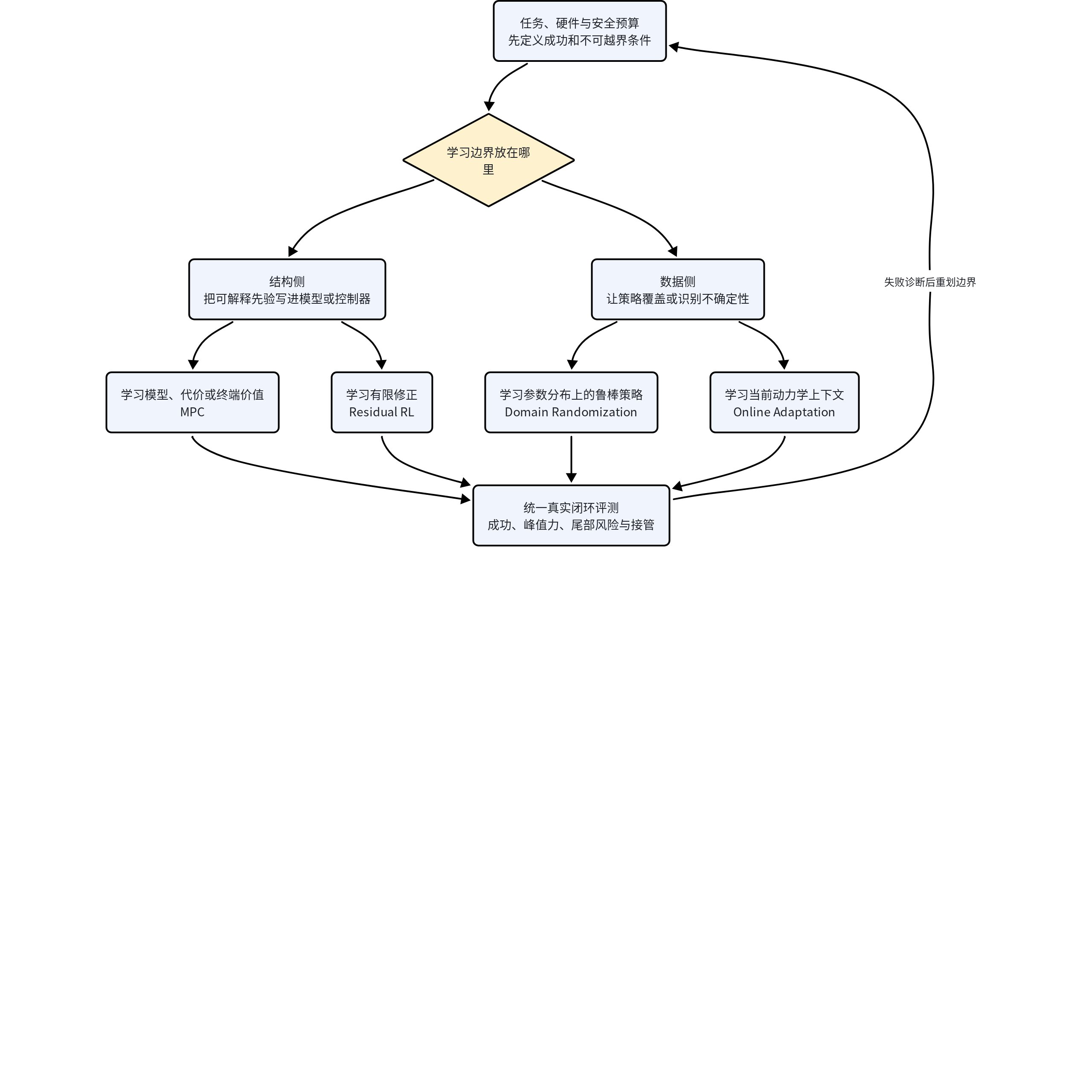
Control and learning are not mutually exclusive choices. The real question is which uncertainties to encode in the model, which structures to embed in the controller, and which remaining regularities to let the system learn from data—and then to use real closed-loop metrics to verify whether this boundary is appropriate.