
Original Feishu Document · Source Revision 30
💡
Track positioning: This chapter belongs to the “Dynamics, Control, and Physical Interaction” track of Physical AI. A learned model decides what to do, while the control system determines how action commands are applied to a real mechanical system stably and safely. Readers need only a foundation in linear algebra, probability and statistics, and basic calculus.
Learning Objectives
After completing this chapter, you should be able to distinguish among kinematics, dynamics, trajectories, and control; verbally interpret the robot dynamics equation; explain the differences among position, velocity, torque, and end-effector delta interfaces; derive the error feedback of PD control; understand impedance control and contact stability; analyze how control latency changes the policy’s data distribution; and design clear control interfaces and real-robot validation procedures for learned policies.
1. What Lies Between Policy Output and Real Motion
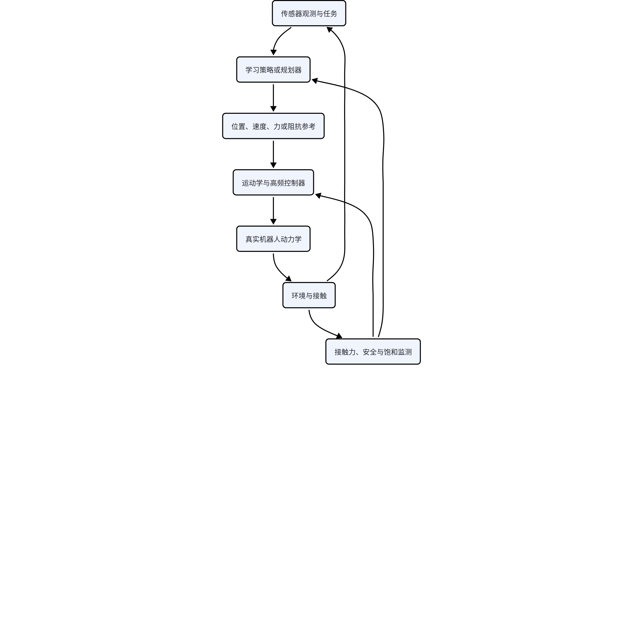
The “action” output by a policy is usually not the final physical quantity applied by the motors. A model may output an end-effector pose delta, inverse kinematics may convert it into joint targets, and a servo controller may then generate currents or torques. Saturation, latency, and errors at any layer will change the actual closed loop.
| Layer | Input | Output | Typical Frequency |
|---|---|---|---|
| Task planning | Language, scene, goal | Subgoal or skill | 0.1-2 Hz |
| Learned policy | Images, proprioceptive state, subgoal | Action chunk or trajectory | 5-50 Hz |
| Motion control | Target position, velocity, force | Joint torque or current | 100-2000 Hz |
| Mechanical system | Torque, external force | Actual pose and contact | Continuous physical process |
2. Kinematics: In Which Coordinate Frame Is an Action Command Expressed?
Let the joint configuration be denoted by . Forward kinematics maps the joint state to the end-effector pose:
Read as: The end-effector pose x is determined by the joint configuration q through the forward-kinematics function f.
Derivation: Starting from the robot base, sequentially compose the rigid-body transformation of each joint to obtain the end-effector transformation; this sequence of matrix multiplications is denoted by the function f. It describes only geometric relationships and does not involve mass, force, or acceleration.
Linearizing for small changes:
Read as: The end-effector velocity equals the Jacobian at the current joint configuration multiplied by the joint velocity.
Derivation: Differentiate the forward kinematics x=f(q) with respect to time. By the chain rule, this yields the product of the partial-derivative matrix J(q) and q_dot. Each column of J represents the instantaneous contribution of unit velocity at the corresponding joint to the end-effector velocity.
Read this as: “The end-effector velocity equals the Jacobian at the current configuration multiplied by the joint velocity.” The Jacobian describes how small motions of individual joints combine to produce end-effector motion.
If the policy outputs an end-effector velocity , one inverse-kinematics solution is:
Read as: The joint-velocity command equals the Jacobian pseudoinverse multiplied by the desired end-effector velocity.
Derivation: Solving the least-squares problem in which J q_dot approximately equals x_dot yields the Moore-Penrose pseudoinverse solution. Near a singular configuration, small singular values amplify commands, so practical systems commonly use a damped pseudoinverse, null-space terms, and velocity limiting.
Here, the pseudoinverse is a least-squares tool that distributes an end-effector velocity requirement across the joint velocities. Near a singular configuration, it may amplify a very small end-effector command into very large joint velocities. Real systems therefore require a damped pseudoinverse, velocity limits, and reachability checks.
3. How to Read the Dynamics Equation
A common form of rigid-body robot dynamics is:
Read as: The sum of the torques required for inertia, joint coupling, gravity, and friction equals the actuator torque plus the torque obtained by mapping external contact forces into joint space.
Derivation: Applying the Lagrangian or Newton-Euler formulation to rigid-body kinetic energy, potential energy, and nonconservative forces yields the internal dynamics terms on the left-hand side. The principle of virtual work maps an external end-effector force through J transpose; under different friction sign conventions, tau_f may instead be moved to the other side of the equation.
| Term | How to Read It | Physical Meaning |
|---|---|---|
| Inertial term | Mass matrix multiplied by joint acceleration | Inertial torque required to produce acceleration |
| Coriolis and centrifugal term | Coriolis and centrifugal term | Coupling torque induced by the state of motion |
| Gravity term | Gravity-compensation term | Torque required to counteract gravity |
| Friction and unmodeled resistance | Friction and unmodeled resistance | Joint friction, cable resistance, and similar effects |
| Actuator torque | Actuator torque | Input that the controller can apply directly |
| External contact force mapped into joint space | External Cartesian force mapped to the joints | Effect of contact forces on the joints |
The complete reading is: “The total torque required for robot acceleration, joint coupling, gravity, and friction equals the actuator torque plus the effect of external contact forces after they are mapped into joint space.” Even if a learned policy does not know each term explicitly, it must handle these effects through data coverage or feedback control.
4. Position, Velocity, Torque, and End-Effector Action Interfaces
| Interface | Model Output | What the Low-Level System Handles | Applicability and Risks |
|---|---|---|---|
| Joint position | Joint-position target | Position servoing and dynamics compensation | Stable and easy to use, but offers limited contact compliance |
| Joint velocity | Joint-velocity target | Velocity tracking and integration | Intuitive for local control, but latency can cause accumulated drift |
| Joint torque | Joint-torque target | Current loop and safety limits | Highly expressive, but imposes stringent data and safety requirements |
| End-effector delta | End-effector pose delta | Inverse kinematics, coordinate transforms, and trajectory smoothing | Clear manipulation semantics, but subject to singularities and unreachability |
| End-effector force or impedance | Desired force or impedance parameters | Force control, impedance control, and contact detection | Suitable for insertion and compliant manipulation, but dependent on force sensing and high-frequency control |
For cross-robot training, action spaces cannot be unified merely by zero-padding. The same token may represent different end-effector velocities, control frequencies, or safety limits on different robots. The coordinate frame, units, normalization method, frequency, and low-level controller must all be recorded.
5. PD Control: The Minimal Feedback Controller
Let the desired position be , with the error defined as:
Read as: The position error equals the desired joint position minus the current joint position.
Derivation: Under this sign convention, a positive error indicates the direction in which the robot has not yet reached the target. If the error is instead defined as q minus q_d, the feedback signs in the subsequent control law must also be changed.
The simplest joint-space PD control law is:
Read as: The control torque consists of proportional feedback on position error, derivative feedback on velocity error, and gravity compensation.
Derivation: The proportional term acts like a spring that pulls the system toward the target, the derivative term acts like a damper that suppresses relative velocity, and gravity compensation offsets the static load. K_p and K_d are usually chosen as positive-definite matrices; saturation, latency, and noise limit the usable gains.
The proportional term generates a restoring torque from the position error, the derivative term provides damping based on the velocity error, and the gravity term offsets the static load. For a one-dimensional mass system , substitution gives:
Read as: Under PD control, the error of a one-dimensional mass satisfies a homogeneous second-order equation composed of mass, damping, and stiffness.
Derivation: Assume the target position is constant. Then q_dot equals negative e_dot, and q_ddot equals negative e_ddot. Substitute the PD torque into m q_ddot equals tau and rearrange to obtain this equation; its characteristic roots determine the convergence speed, oscillation, and damping ratio.
This is equivalent to a damped second-order system. Increasing generally increases stiffness and response speed, while suppresses oscillation. Excessively high gains, however, amplify noise, latency, and unmodeled compliance, causing oscillation or even instability.
6. Impedance Control: Control the Interaction Relationship, Not Just Position
In contact tasks, strict position tracking can generate very large impact forces. Cartesian impedance control aims to make the end effector behave like a virtual spring-damper system:
Read as: The desired end-effector force consists of a virtual spring force generated by position deviation and a virtual damping force generated by velocity deviation.
Derivation: By designing the relationship between the end effector and the target as a spring-damper system, the controller no longer requires rigid trajectory tracking; instead, it specifies how much restoring force should be generated for a given deviation. The contact environment also has stiffness, so closed-loop stability depends on the combined interaction among the robot, controller, sampling process, and environment.
The objective is not to force the end effector to reach a point instantaneously, but to specify how much restoring force should be generated when it deviates from the target. In insertion, wiping, door-opening, and deformable-object manipulation tasks, compliance is often more important than geometric accuracy.
A policy may output a target pose, or it may output stiffness, desired force, or contact phase. Allowing a learned model to output high-frequency torques directly, however, substantially increases safety risks. A more common approach is for the learned policy to provide low-frequency references while a deterministic controller executes high-frequency stabilizing feedback.
7. Contact, Friction, and Mode Transitions
Coulomb friction is commonly approximated using a friction cone:
Read as: The magnitude of the tangential friction force at a contact surface cannot exceed the coefficient of friction multiplied by the normal force.
Derivation: The Coulomb friction model approximates the set of tangential forces that can maintain static contact as a friction cone. Sliding occurs when the required tangential force exceeds this boundary. In three dimensions, f_t is a vector in the tangent plane, and f_n should be a nonnegative normal pressure.
Read this as: “The tangential friction force cannot exceed the coefficient of friction multiplied by the normal force.” If the required tangential force exceeds this boundary, the contact will slide. Successful grasping depends not only on the end-effector position but also on the normal force, coefficient of friction, contact surface, and object inertia.
Contact introduces discrete mode transitions: no contact, initial impact, stable contact, sliding, and separation have different dynamics. A single smooth regression model tends to predict averaged behavior at transition points. Contact-event labels, force sensing, tactile sensing, hybrid dynamics models, or high-frequency feedback are therefore required.
8. Latency, Sampling, and Action Chunks
If the observation latency is , inference time is , and execution communication latency is , the total latency before the action takes effect is approximately:
Read as: The total closed-loop latency approximately equals the sum of observation latency, model-inference latency, and action communication and execution latency.
Derivation: When these three stages occur sequentially, the action is based on information from delta seconds earlier. If the pipeline is parallelized, buffered, or asynchronous, the actual latency also includes queuing and sampling phase. Its distribution should therefore be measured using timestamps rather than represented only by an average.
The policy observes a past state but executes the action in a future state. The higher the speed and the more contact-sensitive the task, the more dangerous this mismatch becomes. Action chunks can reduce the number of inference calls but increase open-loop execution time; frequent replanning improves error correction but may introduce pauses and jitter because of model latency.
| Choice | Benefit | Cost |
|---|---|---|
| Long action chunk | Continuous motion and fewer inference calls | Errors persist longer, and environmental changes are harder to correct |
| Short action chunk | High closed-loop frequency | Increased inference load and boundary jitter |
| Action overlap and smoothing | Reduces abrupt changes at chunk transitions | May delay corrective actions from the new policy |
| Predictive future-state compensation | Reduces latency-induced mismatch | Depends on the accuracy of the world model or state estimator |
9. How Learned Policies and Controllers Should Divide Responsibilities
| Approach | Learned Model Handles | Deterministic System Handles | Applicable Scenarios |
|---|---|---|---|
| Policy outputs position targets | Semantics, scene understanding, and trajectory intent | IK, servoing, speed limits, and safety | General-purpose manipulation and large-scale datasets |
| Policy outputs residuals | Compensation for model error | Baseline control and stability | Fine-grained improvements when a reliable controller is available |
| Policy outputs impedance parameters | Task-dependent compliance adjustment | High-frequency force control | Contact-rich tasks |
| End-to-end torque policy | Complete feedback control | Hardware safety limits | Simulation and high-frequency proprioceptive tasks; caution is required for real-world deployment |
A more end-to-end division of responsibilities is not inherently more advanced. The interface should be selected according to data frequency, sensors, contact risk, and verifiability. Deterministic controllers provide known stable structures, while learned models handle perception, task conditions, and complex residuals that are difficult to model manually.
10. System Identification and Sim-to-Real
Dynamics parameters can be estimated from data. If the model is written as:
Read as: The measurement y_t is written as a linear combination of the known regressor Phi_t and the unknown parameter theta, plus measurement or modeling noise.
Derivation: Many robot dynamics models are linear in mass, inertia, and friction parameters, even when they are nonlinear in the state itself. By stacking equations from multiple time steps, the parameters can be estimated using linear regression; epsilon includes sensor noise and unmodeled dynamics.
Here, contains mass, friction, or motor parameters, and the least-squares estimate is:
Read as: The least-squares parameter estimate equals the inverse from the design matrix’s normal equations multiplied by the observation vector.
Derivation: Minimize the squared error norm, differentiate with respect to theta, and set the gradient to zero to obtain Phi transpose Phi multiplied by theta equals Phi transpose y. A direct inverse exists only when Phi has full column rank; otherwise, a pseudoinverse or regularization should be used, and the condition number and confidence intervals should be reported.
From a statistical perspective, identifiability, noise correlation, and confidence intervals must be examined. Data collected only during slow free-space motion cannot reliably estimate high-speed friction or contact parameters.
Sim-to-real transfer commonly uses system identification, domain randomization, online adaptation, and post-training on real data. A randomization range that is too narrow fails to cover reality, while one that is too broad makes the policy excessively conservative. The key is not to make the simulation look realistic, but to cover the dynamics variables that affect decision-making and control.
11. Real-Robot Evaluation
| Level | Metrics | Question Answered |
|---|---|---|
| Tracking | Position, velocity, and force errors; frequency response | Did the low-level system execute the policy’s commands? |
| Contact | Peak force, slip rate, and time to stable contact | Was the physical interaction safe and stable? |
| Latency | Total perception-to-action latency and jitter | Does the closed-loop timing match the training data? |
| Task | Success rate, completion time, and recovery rate | Did the control modification improve the final behavior? |
| Safety | Collisions, emergency stops, and human intervention rate | Does the average success rate conceal risks? |
12. Chapter Exercises
- Verbally explain every term in the dynamics equation and identify which quantities can typically be measured and which must be estimated.
- Derive the closed-loop PD equation for a one-dimensional mass system, and vary to observe overshoot and convergence time.
- Compare the failure modes of the same policy when using position control versus impedance control for an insertion task.
- Design a latency-sweep experiment that independently varies observation, inference, and execution latency.
- Define a complete action schema for cross-robot data, including coordinate frames, units, frequency, controller, and safety ranges.
- Design a diagnostic experiment that distinguishes a “policy error” from a “controller tracking failure.”
13. Minimal Experiment: How the Policy Interface Changes the Real Closed Loop
First validate kinematics, PD control, and latency in a simulation of a one-dimensional mass or a two-joint manipulator. Then select a repeatable real-world insertion, wiping, or door-opening task. Keep the vision policy and high-level goal fixed, and change only the low-level interface among joint position, joint velocity, end-effector delta, torque, and impedance control.
- Sweep K_p, K_d, impedance stiffness, control frequency, and total latency.
- Introduce errors in mass, friction, extrinsic calibration, and actuator gain, and compare system identification with domain randomization.
- Compute separate error statistics for the pre-contact, initial-impact, stable-contact, and sliding phases.
- Fix the policy output and record the difference between the commanded action and the action actually executed.
- Compare single-step replanning with action chunks of different lengths.
Minimum reporting requirements: Task success rate, tracking error, overshoot, convergence time, peak force, slip rate, energy consumption, saturation ratio, emergency stops, end-to-end latency distribution, and a decomposition of policy errors versus controller tracking errors.
14. Major Failure Modes
| Failure | Symptom | Diagnosis and Correction |
|---|---|---|
| Coordinate-frame or unit error | Reversed direction, abnormal scale, or failure across robots | Explicit from/to frames, units, frequency, and end-to-end calibration |
| Jacobian singularity | A small end-effector command produces enormous joint velocities | Singular values, damped pseudoinverse, null-space control, and limiting |
| Oscillation from high gains and latency | Static tests are normal, but the system diverges at high speed or under network latency | Latency sweeps, frequency response, and gain margin |
| Action saturation | The controller cannot realize the policy command, and errors accumulate over time | Record saturation rate, use anti-windup, and apply reachability filtering |
| Averaging across contact modes | Impacts, stable contact, and sliding are regressed into ambiguous actions | Event labels, hybrid dynamics, and high-frequency feedback |
| Friction-cone violation | The grasp position is correct, but the object slips | Normal force, tangential force, friction margin, and tactile sensing |
| Excessively long open-loop action chunks | The robot continues executing stale actions after a disturbance | Chunk-length sweeps, asynchronous replanning, and interruption mechanisms |
| Unidentifiable system identification | Parameter fitting error is low, but the model fails on a different trajectory | Excitation coverage, design-matrix condition number, and confidence intervals |
| Incorrect simulation randomization range | Too narrow to cover reality, or so broad that the policy becomes excessively conservative | Real-world residuals, parameter sensitivity, and per-variable randomization ablations |
15. Paper Facts, Author Interpretations, and Course Assessments
| Work | Paper Facts | Author Interpretation | Course Assessment |
|---|---|---|---|
| Operational Space Control | Constructs dynamics and control laws in task space and maps end-effector task forces to joint torques | A robot’s dynamic behavior can be designed directly around end-effector tasks | Provides a foundation for contact and task-space control, but depends on models, state estimation, and a stable implementation |
| Residual RL | Allows a learned policy to add residuals to the actions of an existing controller, using prior structure while correcting model errors | Deterministic control and learned residuals can complement each other | Deployability depends on the residual range, safety constraints, and baseline-controller quality; final reward alone is insufficient |
| Domain Randomization | Randomizes visual or dynamics parameters in simulation to improve coverage of the real-world distribution | Sufficiently diverse simulations can make reality part of the training distribution | Randomized variables must match control sensitivity, and the ranges must be validated against real-world residuals |
| Dactyl | Combines large-scale simulation randomization and reinforcement learning to perform real-world dexterous hand manipulation | Complex contact skills can transfer through simulation scale and randomization | It demonstrates the feasibility of a particular systems-engineering approach, but does not imply that every task can be solved by broader randomization |
16. Cross-Reading for This Course
F1|Feedback Control and Stability
F2|Contact, Impedance, Force Control, and Tactile Sensing
F3|System Identification, Latency, and Sim-to-Real
F4|Humanoids, Locomotion, and Whole-Body Control
Required Conclusions from This Chapter
- A policy output is not the endpoint of a physical action; it is a reference input to the control system.
- The action interface determines the data distribution, cross-robot semantics, and safety boundaries.
- Contact, latency, and low-level control change the closed-loop distribution that the learned policy actually encounters.
- World models, VLAs, and hierarchical planning must ultimately undergo real-world validation through dynamics and control.
- For real robots, a well-designed combination of stable structures and learning capabilities is generally preferable to an unverifiable fully end-to-end stack.