Original Feishu Document · Source Revision 21

💡

Mechanisms Lesson: A learning policy outputs reference actions, and a feedback controller converts those references into stable motion. Starting from linear state-space models, closed-loop poles, PD control, discrete sampling, saturation, and Lyapunov intuition, this lesson establishes the interface between policies and controllers.

Learning Objectives

After completing this lesson, you should be able to write a state-space model; explain open-loop and closed-loop control; derive the second-order PD error equation; determine linear stability from eigenvalues; analyze discrete sampling, delay, saturation, and action smoothing; and distinguish policy errors from control tracking errors.

1. State Space

Linear system:

Interpretation: The rate of change of the state equals the sum of the system's autonomous evolution A x and the effect of the control input B u.

Derivation: Take a first-order Taylor expansion of the nonlinear dynamics around an operating point. The constant term cancels at the equilibrium point, while the first-order partial derivatives with respect to the state and input form A and B, respectively. This model is only approximately valid near the operating point.

Interpretation: The measurable output y is a linear projection of the internal state x through the matrix C.

Derivation: Sensors usually observe only part of the state or a linear combination of state variables. To avoid an algebraic loop caused by the control input directly entering the output, this lesson assumes D equals zero. If y=Cx+Du, D must be handled separately when substituting the closed-loop control law.

Here, x denotes the internal state, u denotes the control input, and y denotes the measurable output. Nonlinear robot dynamics can be linearized around a selected operating point, but the valid range of the linear model must be verified through perturbation and trajectory tests.

2. Open-Loop and Closed-Loop Control

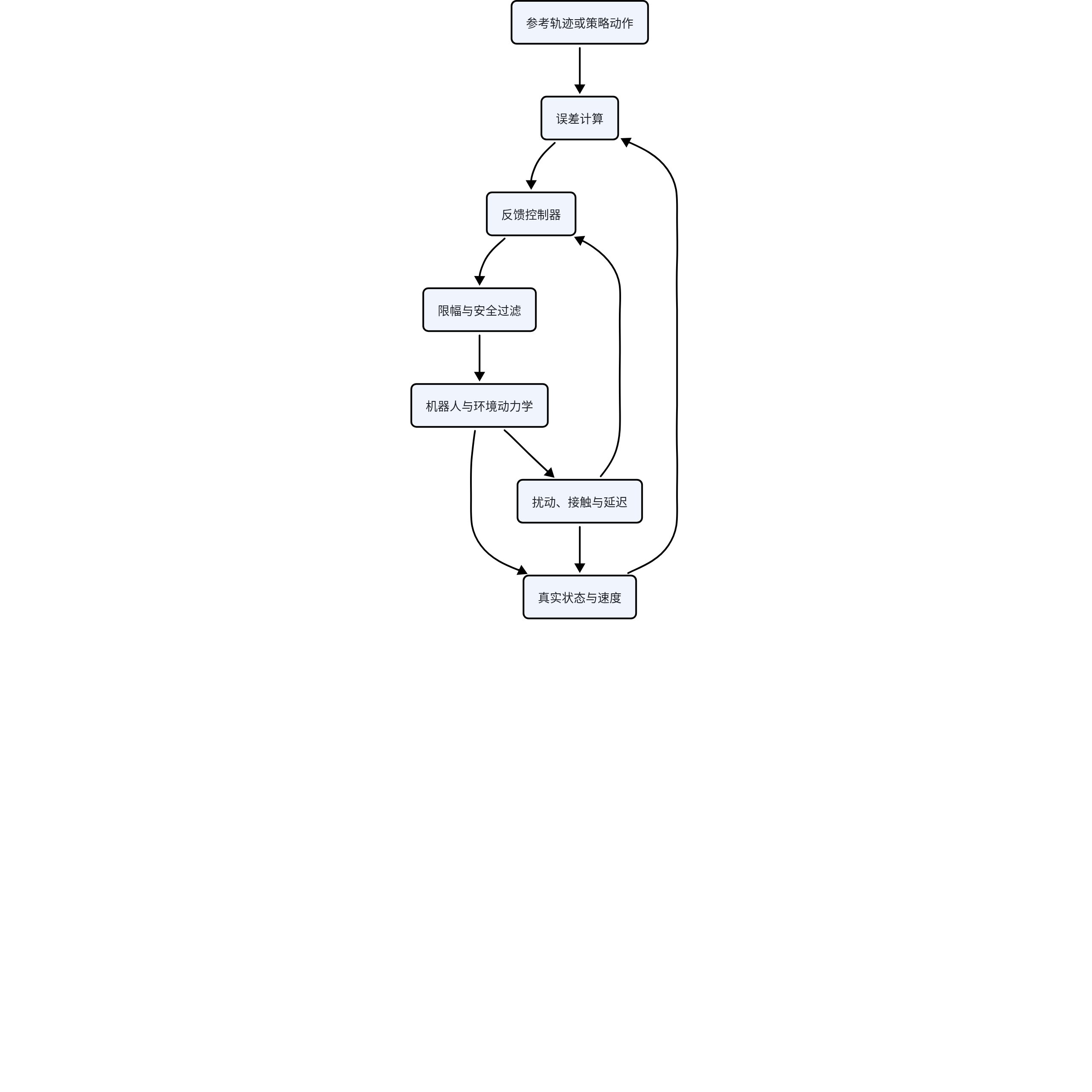
Open-loop control applies inputs solely according to a predefined plan; closed-loop control uses the error:

Interpretation: The control input equals the gain K multiplied by the error between the reference output and the actual output.

Derivation: Negative feedback produces a corrective input when the output is below the reference and a correction in the opposite direction when the output is above the reference. K may be a scalar or a matrix. If the sign convention changes, the closed-loop matrix must be changed accordingly.

Substitution gives:

Interpretation: The closed-loop state evolves according to the modified system matrix A minus BKC and is driven by the reference input BKr.

Derivation: Given y=Cx and u=K(r-y), substitute u into A x+B u, expand the expression, and collect the x terms. For a zero reference, the real parts of the eigenvalues of A-BKC determine the local stability of the continuous-time linear closed-loop system.

A continuous-time linear system is locally asymptotically stable when the real parts of the eigenvalues of the closed-loop matrix are negative.

3. One-Dimensional PD Derivation

Mass system:

Interpretation: The mass m multiplied by the acceleration of a one-dimensional mass equals the control force u.

Derivation: This is the minimal model obtained from Newton's second law by neglecting friction, gravity, and external forces. It is used to illustrate the feedback structure and does not represent complete robot joint dynamics.

Control law:

Interpretation: The PD control input is the sum of the position error multiplied by the proportional gain and the velocity error multiplied by the derivative gain.

Derivation: The proportional term provides a restoring force, while the derivative term provides damping. When K_p and K_d are positive, they produce spring-damper behavior around a fixed target. In practice, actuator saturation and sampling delay limit the usable gains.

With a fixed target, define the error :

Interpretation: When the error e is defined as the current position minus the target position, the PD closed-loop error satisfies the standard homogeneous second-order equation.

Derivation: For a fixed target, e_dot=q_dot and e_ddot=q_ddot. Substitute q_d-q=-e and negative q_dot into the control law, then substitute the result into m q_ddot=u and rearrange the terms.

Natural frequency and damping ratio:

Interpretation: The closed-loop natural frequency is the square root of K_p divided by the mass, and the damping ratio is K_d divided by twice the square root of mK_p.

Derivation: Divide the error equation by m and compare its coefficients with the standard second-order form e_ddot+2 zeta omega_n e_dot+omega_n squared e=0 to obtain the two expressions.

The proportional gain primarily determines the effective stiffness and response speed, while the derivative gain primarily provides dissipation and suppresses oscillation. Excessively high gains amplify measurement noise, delay, actuator compliance, and unmodeled high-frequency modes.

4. Discrete Time

In practice, the controller updates at the period :

Interpretation: The next state of the discrete-time system is computed from the current state and current control input through the discrete matrices A_d and B_d.

Derivation: Holding the input constant over the sampling period Delta t and integrating the continuous-time linear system gives A_d=e^{A Delta t}, while B_d is obtained from a matrix-exponential integral. Discrete-time stability requires the magnitudes of the closed-loop eigenvalues to be less than one.

Discrete-time stability requires the closed-loop eigenvalues to lie inside the unit circle. The same PD gains behave differently at 1 kHz and 20 Hz.

5. Delay

Delayed control:

Interpretation: The controller computes the current input from the reference and output error measured delta seconds earlier.

Derivation: Observation, computation, and communication mean that the controller can only access past information. In the frequency domain, a pure delay introduces phase lag that increases with frequency, thereby reducing the stability margin. Actual delay should be modeled using timestamp distributions rather than a single average value.

Delay increases phase lag and reduces the stability margin. VLA inference time, network communication, and action chunks all contribute to the total delay.

6. Saturation and Anti-Windup

Actuators are subject to:

Interpretation: The control input must lie between the minimum and maximum values permitted by the actuator.

Derivation: Current, torque, velocity, and travel all have physical limits, and commands exceeding those limits are clipped. Clipping is nonlinear and changes the linear closed-loop behavior. If an integral term is also present, persistent error accumulates and causes windup, so anti-windup is required.

Saturation invalidates linear analysis. Integral controllers experience windup during saturation and therefore require anti-windup. Learning policy outputs must also remain within physical limits after action normalization and decoding.

7. Lyapunov Intuition

Suppose an energy function exists:

Interpretation: The Lyapunov function is zero at the equilibrium point, positive at all other states, and strictly decreases along every non-equilibrium trajectory.

Derivation: V can be interpreted as a generalized energy. If every state away from equilibrium has positive energy and the system's motion continuously dissipates energy, the trajectory cannot remain indefinitely at a nonzero energy level. The equilibrium is therefore asymptotically stable. If the derivative is only negative semidefinite, additional conditions such as LaSalle's invariance principle are required.

The system state converges to the equilibrium point. For the PD-controlled mass system, choose:

Interpretation: The candidate Lyapunov function consists of a kinetic-energy term for the error velocity and a virtual spring potential-energy term for the position error.

Derivation: The kinetic energy of the mass system is one-half m times e_dot squared. Proportional control is equivalent to a spring with stiffness K_p, whose potential energy is one-half K_p times e squared. When m and K_p are positive, V is positive definite with respect to the error state.

Differentiating gives:

Interpretation: The rate of change of the Lyapunov function equals the negative derivative gain multiplied by the squared error velocity, so it cannot increase.

Derivation: Differentiating V gives m e_dot e_ddot+K_p e e_dot. Substituting the PD error equation for m e_ddot causes the spring terms to cancel, leaving only negative damping dissipation. When V_dot is zero, e_dot=0; together with the dynamics, LaSalle's invariance principle can be used to show that e ultimately converges to zero.

This explains how the derivative term dissipates energy.

8. Trajectory Tracking

The policy outputs an action chunk . The controller tracks each reference point. Check whether:

• The reference trajectory is continuous and reachable.
• Velocity and acceleration limits are respected.
• Discontinuities occur at chunk boundaries.
• Tracking errors are fed back to the policy.

9. Policy–Controller Interface

Policy Output	Controller	Risk
Joint position	Position PD	Rigid contact
Joint velocity	Velocity servo	Integration drift
End-effector pose	IK + position control	Singularities and unreachable poses
Torque	Current loop	Safety and high-frequency requirements
Impedance parameters	Force/impedance control	Stability and sensing

10. Diagnostic Experiments

1. Record the target actions and actual trajectories.
2. Measure the controller's tracking error separately.
3. Simulate the policy using an ideal controller.
4. Hold the policy fixed while sweeping gains and frequencies.
5. Hold the controller fixed while comparing different policies.
6. Inject delay, noise, and saturation.

11. Lesson Exercises

1. Derive the damping ratio for PD control.
2. Calculate the discrete closed-loop eigenvalues.
3. Use a Lyapunov function to explain PD stability.
4. Design a chunk-boundary smoother.
5. Explain why a high policy success rate may conceal controller instability.
6. Distinguish model inference delay from actuator delay.

12. Minimal Experiment: Stability, Sampling, and the Policy Interface

Start with a one-dimensional mass and an inverted pendulum or two-joint robotic arm. Fix the reference trajectory, then separately implement a continuous-time approximation, discrete-time PD control, delayed control, saturation, and anti-windup. Next, have the same learning policy output the reference trajectory while keeping the controller replaceable.

1. Sweep K_p, K_d, the sampling period, and delay; plot the closed-loop poles, overshoot, and settling time.
2. Compare the theoretical discrete-time model with trajectories obtained using actual timestamps.
3. Inject action saturation, sensor noise, and discontinuities at chunk boundaries.
4. Hold the policy fixed while replacing the controller, and hold the controller fixed while replacing the policy, to separate the two types of errors.
5. Add a safety filter and compare the unmodified policy actions with the actions actually executed.

Minimum reporting requirements: closed-loop eigenvalues, change in the Lyapunov candidate, tracking error, overshoot, settling time, saturation rate, action modification rate, end-to-end delay, task success rate, and safety violations.

13. Major Failure Modes

Failure	Symptom	Diagnosis and Correction
Stable in continuous time but unstable in discrete time	Theoretical gains cause oscillation in a low-frequency controller	Examine discrete poles, actual sampling jitter, and the zero-order-hold model
Insufficient delay margin	Minor inference or network delay amplifies overshoot	Perform delay sweeps and examine phase margin and predictive compensation
High gains amplify noise	Tracking becomes faster, but motor vibration, energy consumption, and wear increase	Examine velocity-estimation noise, filtering, and the control spectrum
Saturation and windup	Recovery is slow or severe overshoot occurs after commands remain beyond the limits for an extended period	Compare commanded and actual actions, inspect the integral state, and apply anti-windup
Infeasible reference trajectory	The controller is stable but can never catch up with the policy output	Enforce velocity, acceleration, jerk, and reachability constraints
Chunk-boundary discontinuities	Adjacent action chunks produce velocity or force spikes at their junction	Check boundary continuity, interpolation, and online interruption and replanning
Misapplication of Lyapunov conditions	Strict convergence is claimed after proving only that V_dot is less than or equal to zero	Check the invariant set, LaSalle conditions, and the model's domain of validity
Safety filter conceals policy defects	The task succeeds, but the filter modifies most actions	Report the action modification rate and unfiltered counterfactuals, and retrain the policy

14. Paper Facts, Authors' Interpretations, and Course Assessments

Approach	Paper Facts	Authors' Interpretation	Course Assessment
LQR / linear control	Optimal state feedback is obtained under linear dynamics and a quadratic cost, and the closed-loop poles can be analyzed	Model structure can provide interpretable trade-offs between stability and performance	It provides a local foundation but does not cover strong contact, multimodal observations, or large-range nonlinearities
Control Barrier Function	Online optimization constrains the system to remain within a safe set and can be combined with a nominal controller	Safety constraints can be implemented as a control-layer filter independently of the policy	Safety guarantees depend on the dynamics model, relative degree, and feasibility; the filter modification rate and failure conditions should be reported
Residual RL	A learning policy adds a residual to an existing controller to correct model errors or complex dynamics	Stability priors and learning capabilities can complement each other	Residual bounds, exploration safety, and the quality of the baseline controller must be included in the evaluation
Action chunk policy	Predicting multiple actions at once can reduce inference frequency and exploit temporal correlations	Action chunks support long-horizon continuous control	Longer chunks create greater open-loop risk; delay, boundary continuity, and the ability to interrupt in response to disturbances must be measured

15. Cross-Reading

F0｜Dynamics, Control, and Physical Interaction

F2｜Contact, Impedance, Force Control, and Tactile Sensing

F3｜System Identification, Delay, and Sim-to-Real