

Original Feishu Document · Source Revision 35
💡
Mechanisms lesson: The difference between simulation and the real world is not an abstract “domain gap,” but the combined error arising from mass, friction, compliance, actuators, sensors, latency, and unmodeled disturbances. This lesson decomposes these errors into objects that can be measured, estimated, randomized, and compensated for.
Learning Objectives
After completing this lesson, you should be able to build a parameterized dynamics model; derive least-squares system identification; explain identifiability, persistent excitation, and closed-loop bias; calculate the phase loss caused by latency; and distinguish among domain randomization, online adaptation, residual learning, and digital twins.
1. What System Identification Estimates
Write the dynamics in parameterized form:
Interpretation: The next state is jointly determined by the current state, control input, and physical parameters through the dynamics function, with process noise and unmodeled disturbances added.
Derivation: Integrating the continuous-time dynamics over one sampling period yields a discrete state transition. Mass, inertia, friction, and actuator parameters are placed in theta; discretization errors, external disturbances, and effects not explicitly modeled are grouped into w_t. The goal of identification is to reduce uncertainty in theta using data, not to assume that w_t will disappear automatically.
Slowly varying, reusable physical parameters should be separated from fast, unpredictable disturbances. If all errors are absorbed into the parameters, the estimates will drift across data segments; if all errors are treated as noise, neither the simulator nor the controller can be calibrated.
The purpose of identification is not to pursue a perfect physical truth, but to obtain a model that is sufficiently useful for control and prediction and whose uncertainty can be characterized.
2. Linear Regression Form and Least Squares
Many rigid-body dynamics equations can be rearranged as:
Interpretation: The quantity measured at time t equals a known regression matrix multiplied by unknown parameters, plus measurement error.
Derivation: Although many rigid-body inverse dynamics models are nonlinear in the state, they can be rearranged to be linear in physical parameters such as mass, inertia, and friction coefficients. Place the known terms constructed from position, velocity, acceleration, and input in Phi_t, and place the physical coefficients to be estimated in theta, yielding a linear parameter regression.
Stacking samples from multiple time steps row by row produces a unified regression problem. The next step is to minimize the squared residuals over all samples to find the parameters that best explain the data.
Interpretation: The parameter estimate is the set of parameters that minimizes the sum of squared prediction residuals over all samples.
Derivation: After stacking the regression equations from each time step, the residual is y-Phi theta. If the errors are independent, zero-mean, and have the same Gaussian variance, maximizing the data likelihood is equivalent to minimizing the sum of squared residuals; if the noise variances differ or the noise is correlated, weighted least squares should be used instead.
Differentiate the objective and set the result to zero:
Interpretation: The gradient of the residual sum of squares with respect to the parameters equals negative two times the transpose of the regression matrix multiplied by the residual; at the optimum, this gradient is zero.
Derivation: Expanding the quadratic objective gives y transpose y minus two times theta transpose Phi transpose y, plus theta transpose Phi transpose Phi theta. Differentiating each term with respect to theta and setting the result to zero yields the normal equations.
Only when the information matrix has full rank and is numerically well-conditioned is every parameter direction sufficiently constrained by the data, giving the closed-form solution a clear identification meaning.
Interpretation: When the information matrix is invertible, the least-squares parameter estimate is given by the closed-form solution to the normal equations.
Derivation: Setting the gradient to zero gives Phi transpose Phi times theta equals Phi transpose y. If Phi transpose Phi is full-rank and invertible, left-multiplying both sides by its inverse yields the solution. If the matrix is singular or ill-conditioned, a pseudoinverse, regularization, or redesigned excitation should be used; the numerical result must not be treated as an identified physical ground truth.
If the robot performs only one type of slow motion, inertial effects may be weak, while friction and payload effects may compensate for each other. In that case, even if the trajectory fit is excellent, the individual physical parameters may not have been genuinely distinguished.
3. Identifiability and Persistent Excitation
Identifiability asks whether different parameters produce distinguishable effects in the observations. Persistent excitation requires the input to cover sufficiently rich frequencies and directions so that the information matrix:
Interpretation: Under equal-variance Gaussian noise, the Fisher information matrix for the parameters equals the transpose of the regression matrix multiplied by itself, divided by the noise variance.
Derivation: The second-order curvature of the log-likelihood for Gaussian regression is determined by Phi transpose Phi; the lower the noise, the more information each data sample carries. Small eigenvalues correspond to parameter directions that are barely excited, while a large condition number means that some parameter combinations are difficult to distinguish.
is well-conditioned. Random motion is not necessarily good excitation: it may reach safety boundaries while still failing to cover critical operating regions. Better experiments use multisine, chirp, or task-relevant trajectories designed to remain within safe limits.
4. Why Closed-Loop Data Can Produce Bias
The controller changes its input in response to measurement noise, so may be correlated with the noise. Ordinary least squares assumes that the regressors and errors are independent, but this condition may not hold under closed-loop operation. Solutions include instrumental variables, prediction-error methods, joint state-parameter estimation, or dedicated open-loop identification experiments.
5. Latency Is Not Merely “Being a Little Slower”
Total closed-loop latency can be decomposed as:
Interpretation: The closed-loop latency of a feedback sample, from the physical event to the actuator response, is composed of the time spent in stages such as perception, encoding, inference, communication, and actuation.
Derivation: Record timestamps stage by stage along the causal chain of the same sample. Summing the time differences between adjacent stages telescopes to the final execution time minus the initial perception time. Pipeline parallelism does not mean that an individual sample has no latency, so queuing and jitter must also be measured separately.
A pure delay contributes the following in the frequency domain:
Interpretation: A pure delay of duration tau is equivalent in the Laplace domain to multiplication by the exponential factor e raised to negative s tau.
Derivation: If the output is a time-shifted version of the input, namely y(t)=x(t-tau), the time-shift property of the Laplace transform gives Y(s)=e^{-s tau}X(s). Therefore, the transfer function of a pure delay is this exponential term.
Along the frequency response, a pure delay does not change the amplitude of a sinusoidal signal, but it introduces a phase lag that increases linearly with frequency.
Interpretation: After a signal with angular frequency omega passes through a pure delay, the additional phase lag equals the negative angular frequency multiplied by the delay duration.
Derivation: Substituting j omega for s gives e raised to negative j omega tau. By Euler’s formula, its magnitude is one and its phase angle is negative omega tau. Thus, a delay does not attenuate the amplitude of a sinusoid, but it directly consumes phase margin.
For example, 10 Hz motion corresponds to an angular frequency of approximately 62.8 rad/s; a 50 ms pure delay introduces approximately -3.14 rad, or -180 degrees, of additional phase. In practice, the closed loop will become unstable before reaching this extreme because its existing phase margin will already have been exhausted. Therefore, “the average latency is only tens of milliseconds” is not a sufficient safety assessment.
💡
Interactive Validation|Feedback Control, Contact, and Sim-to-Real Laboratory
Vary the feedback gain, latency, and domain-randomization coverage to observe the trade-offs among closed-loop stability, contact overshoot, and real-world transfer robustness.
Feedback Control, Contact, and Sim-to-Real Laboratory
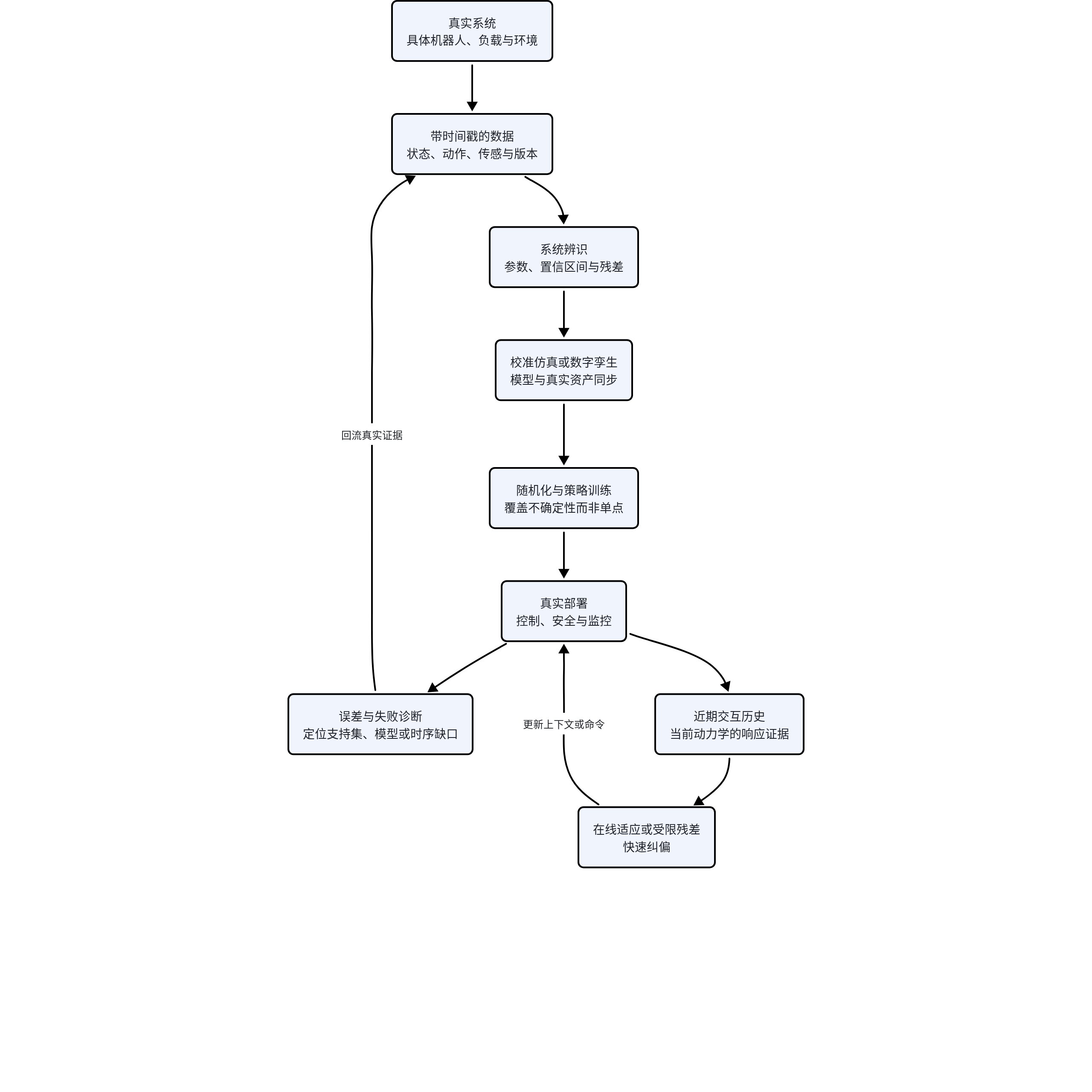
:::6. Five Main Approaches to Sim-to-Real
| Approach | What Is Learned or Adjusted | Applicable Conditions and Key Validation |
|---|---|---|
| System identification | Model parameters such as mass, inertia, friction, actuators, and latency | The model structure is credible and the parameters are observable; identifiability, confidence intervals, and cross-trajectory prediction errors must be reported |
| Domain Randomization | A policy robust to a distribution of parameters | The randomization support covers the real system; in-distribution, boundary, and out-of-distribution conditions must be tested separately |
| Online adaptation | A dynamics context or rapidly estimated parameters inferred from recent history | Distinguishable response differences exist during deployment; history permutation, parameter-shift, and adaptation-time tests are required |
| Residual learning | Bounded corrections not explained by the baseline model or controller | A stable baseline exists and the residual is constrained; degradation with the residual disabled and out-of-bounds protection must be validated |
| Digital twin | Model state continuously synchronized with a specific asset, calibration, clock, software version, and operational data | Long-term operations, maintenance, diagnostics, and replay are required; model updates must be shown to be traceable, and a one-off offline high-fidelity simulation must not be mislabeled as a twin |
A digital twin is not a fifth type of neural network. It is a continuously updated engineering object that links system identification, asset identity, time synchronization, parameter versions, simulation, and evidence from real-world operation. If a high-fidelity simulator cannot specify which robot, firmware version, calibration, and data segment it corresponds to, it is merely a simulator, not an auditable digital twin.
7. Statistical Interpretation of Domain Randomization
The training objective can be written as:
Interpretation: Select a policy that maximizes the average return across dynamics environments sampled from the training parameter distribution.
Derivation: Treat the unknown real dynamics as parameter-valued random variables. During training, repeatedly sample parameters from p_train and estimate the return; the sample mean of the returns is a Monte Carlo estimate of this expectation. This objective optimizes the mean over the training distribution; it does not automatically control out-of-distribution systems or low-probability tail failures.
This objective guarantees only average performance over the training parameter distribution. If the randomization is too narrow, it may fail to include the real system. If it is too broad, much of the training budget will be spent on combinations that cannot occur, potentially forcing the policy to become excessively conservative.
A risk-sensitive version can optimize a lower quantile or the worst case:
Interpretation: Select a policy that maximizes the average return under the worst alpha fraction of dynamics conditions.
Derivation: First sort the parameter samples by return from lowest to highest, then average the lowest alpha fraction. This is the lower-tail CVaR convention used in this lesson. It concentrates gradient pressure on tail failures, but still depends on whether the training distribution covers the real risks.
This objective focuses more on failures in the parameter-distribution tail rather than only improving average return.
8. Online Adaptation and Latent Variables
Estimate the dynamics context from recent history:
Interpretation: The adaptation encoder compresses a recent history of observations and actions into the current dynamics context z_t.
Derivation: Mass, payload, friction, and actuator state are usually not visible in a single-frame observation, but they leave evidence in the system’s response after a sequence of actions. By treating these hidden parameters as partially observable state, the history encoder approximates a summary of their posterior. It can be trained using supervision from privileged parameters or learned end to end using only policy return or prediction loss.
The deployed policy is conditioned on both the current observation and the dynamics context. The context does not necessarily correspond to an interpretable mass or friction value; it only needs to preserve response information useful for behavior. The real test is whether the system can recover quickly from abrupt parameter changes, payload changes, and new hardware—not whether visualizations of the latent space appear clustered.
9. The Trade-off Between Action Chunks and Latency
Long action chunks reduce inference calls and network jitter, but increase the open-loop duration between feedback-driven replanning events. Suppose the model predicts H steps each time but executes only the first h steps:
Interpretation: The replanning period equals the number of action steps actually executed multiplied by the control interval per step, and the number of executed steps cannot exceed the current prediction length.
Derivation: Adjacent control commands are separated by Delta t. The policy is invoked again only after h commands have been executed consecutively, so h sampling periods elapse between two replanning events. H determines the available prediction horizon, while h determines the actual open-loop duration. Increasing H does not necessarily reduce the feedback frequency; increasing h does.
When selecting h, inference throughput, the rate of environmental change, the frequency of contact events, and closed-loop recovery requirements must all be considered. In engineering reports, the prediction length, execution length, and end-to-end latency should be recorded separately; reporting only the “chunk size” is insufficient.
10. Minimal Experiment
Plant. Simulate a one-dimensional cart whose real parameters include mass, Coulomb friction, viscous friction, a first-order actuator time constant, sensor low-pass filtering, and variable latency. During simulation training, only the training distribution may be accessed. The test script stores the real parameters separately to prevent implicit leakage.
| Experimental Stage | Setup | Question to Answer |
|---|---|---|
| Identification excitation | Constant velocity, single-frequency sine, multisine, chirp, and task trajectories | Which parameter directions were not excited? Does the condition number agree with the parameter error? |
| Closed-loop data | Safe open-loop trajectories, closed-loop control trajectories, and estimation with instrumental variables | Does ordinary least squares become biased because the input is correlated with noise? |
| Policy approach | Nominal model, identification-based calibration, randomization, history-based adaptation, and constrained residuals | Does performance come from a more accurate model, distributional robustness, rapid inference, or a correction interface? |
| Test stratification | Inside the training distribution, at the support boundary, out of distribution, and with abrupt parameter changes during operation | Can average generalization, tail robustness, and online recovery be distinguished? |
| Latency sweep | Hold average latency fixed while independently varying jitter, dropped frames, and the replanning period | Is closed-loop failure actually caused by average latency, variance, or the open-loop action-chunk length? |
Measurements. During identification, report parameter bias, confidence-interval coverage, information-matrix condition number, one-step prediction error, and long-horizon rollout error. During control, report average return, worst-10% return, out-of-bounds rate, settling time, and the physical time required to adapt to new parameters.
Key ablations. Freeze the adaptation context, shuffle the history order, misalign timestamps, move the real parameters outside the randomization support, and progressively relax the residual-amplitude limit. Each ablation should change only one mechanism, so that it is possible to determine whether the model is identifying the dynamics, memorizing the task phase, or relying on the baseline controller as a fallback.
11. Failure Modes
| Failure Mode | Observable Symptom | Root Cause | Validation and Remedy |
|---|---|---|---|
| Real parameters lie outside the randomization support | Performance is stable within the training distribution but suddenly falls off a cliff beyond the boundary | The support was defined using arbitrary ranges and omitted actuator or latency coupling | Plot parameter-conditioned performance surfaces; update the ranges using real data; retain out-of-distribution tests |
| Parameters are unidentifiable | Fitting error is small, but parameter estimates vary dramatically across data segments | Insufficient excitation, or multiple parameters affect observations only through a combined form | Inspect singular values and the condition number; redesign multisine or task-relevant excitation |
| Observation pipelines are inconsistent | A policy performs well with simulator states but becomes unstable after real filtering and timestamps are introduced | Training did not simulate low-pass filtering, quantization, dropped frames, buffering, and latency jitter | Include the complete observation pipeline in replay and randomization; sweep latency components individually |
| Residual overrides the baseline | Residual amplitude remains saturated, and behavior changes little when the baseline is disabled | The learner has effectively relearned the entire controller, losing structural protection | Constrain residual amplitude, rate of change, and energy; report the residual as a fraction of the total command |
| Adapter confounds task and dynamics | The latent representation shifts when the target changes but responds slowly to an abrupt payload change | The history contains both task-phase and dynamics information, while the supervision target is insufficient | Cross-combine tasks and parameters; perform history permutation; add a privileged dynamics teacher or disentanglement loss |
| Mean performance masks tail collapse | The mean improves, but high-cost instability occurs in a small number of parameter regions | Training and reporting optimize only expected return | Report worst-case quantiles, CVaR, out-of-bounds rate, and parameter-conditioned curves |
12. Exercises
- Derive the normal equations from the least-squares objective.
- Explain why a single constant-velocity trajectory makes it difficult to identify both mass and Coulomb friction.
- Calculate the phase loss for 10 Hz motion under 50 ms of latency.
- Design a randomization distribution covering mass, friction, visual latency, and actuator gain.
- Compare the most critical validation sets for system identification, randomization, and online adaptation.
Relationship to Other Tracks
The world model learned in Track B can also be used for dynamics prediction, but F3 places greater emphasis on controllability, identifiability, and real-world latency. The policy interfaces in Tracks A and D determine whether errors can be absorbed by the low-level controller. Track G maintains the evidence chain for parameters, firmware, latency, and data versions.
13. Paper Evidence Matrix
Sim-to-Real literature often treats “extensive randomization” or “rapid adaptation” as directly equivalent to “real-world reliability.” The table below separates experimental facts, the authors’ mechanistic explanations, and the lesson’s assessment.
| Work | Facts Reported in the Paper | Authors’ Explanation | Lesson Assessment |
|---|---|---|---|
| Ljung|System Identification | System identification theory systematically addresses model structure, experimental design, prediction error, closed-loop data, and estimation uncertainty. | The author treats identification as a joint problem involving “data, a model set, and a selection criterion,” rather than merely applying a least-squares formula. | Low parameter-fitting error does not mean the model is suitable for control; identifiability, residual structure, and task-relevant prediction must also be validated. |
| Peng et al.|Dynamics Randomization | This work randomizes dynamics parameters during simulation training and transfers the policy to real robot-control tasks. | The authors use parameter variation to force the policy to learn behavior that is insensitive to model error rather than relying on a single nominal model. | The key to effective randomization is not making the ranges as broad as possible, but ensuring that the support, joint correlations, and coverage of the real system are credible. |
| Chebotar et al.|SimOpt | SimOpt iteratively adjusts the simulator parameter distribution using discrepancies between real and simulated trajectories, forming a closed-loop calibration process. | The authors use a small amount of real-world experience to update the randomization distribution rather than relearning the entire policy directly on the real robot. | This identifies a distribution rather than only a point estimate of the parameters; evaluation must prevent the real-world calibration set from being mixed with the final test set. |
| Kumar et al.|Rapid Motor Adaptation | RMA uses recent interaction history to infer environmental context and demonstrates rapid adaptation to terrain and dynamics changes on a quadruped robot. | The authors divide deployment into a base policy and an adaptation module. Privileged environment information can be used during training, while only historical observations are used during deployment. | Whether the latent representation forms clusters is unimportant; the key evidence is recovery time after abrupt parameter changes, degradation under history permutation, and testing on new hardware. |
| Johannink et al.|Residual RL | Residual RL learns corrections on top of an existing controller and is applied to real-world contact-rich tasks. | The authors use the prior controller to handle the components that are easy to model and use learning to address the remaining errors. | The residual approach retains engineering significance only when its amplitude, energy, and safety boundaries are controlled; otherwise, it is merely end-to-end control behind a different interface. |
14. Cross-Reading
Read together with F1 and F2. Identification errors and latency ultimately manifest through stability margins, peak forces, and contact oscillations. Model-prediction errors must be evaluated against closed-loop metrics rather than only offline losses.
Read together with Track A. Action chunks can reduce inference-call frequency but extend the open-loop execution window. The VLA action interface determines whether latency and model error are handled by the policy or the low-level controller.
Read together with Track B. World models learn high-dimensional latent dynamics, while system identification emphasizes excitation, verifiability, and uncertainty. The two can share data, but visually impressive video predictions cannot replace control-relevant validation.
Read together with Track G. A genuine digital twin depends on an evidence chain covering robot identity, calibration, firmware, clocks, data, and parameter versions. Without this system information, Sim-to-Real results are neither reproducible nor sufficient for localizing regressions.