

Original Feishu Document · Source Revision 23
💡
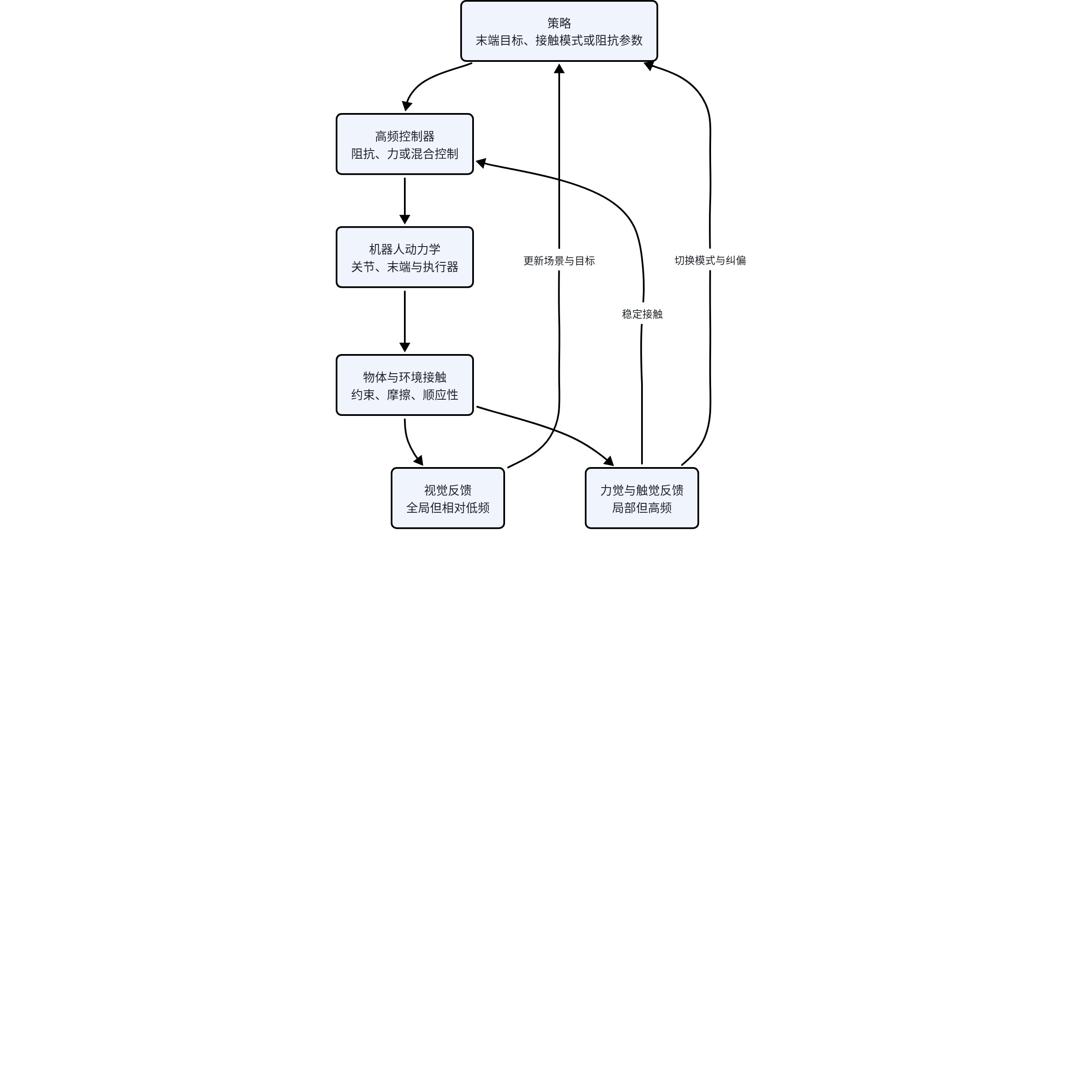
Mechanisms lesson: In free space, a position error usually means “the robot has not reached the target yet.” After contact occurs, the same position error may mean “the robot is pushing harder and harder against the environment.” This lesson examines how policies, controllers, sensors, and contact dynamics form a stable physical closed loop.
Learning Objectives
After completing this lesson, you should be able to interpret equations for contact constraints, friction cones, force control, and impedance control; derive the equivalent stiffness for one-dimensional environmental contact; explain why tactile sensing is not merely an additional input channel but a high-frequency observation of contact state; and design a minimal experiment for insertion, wiping, or compliant grasping.
1. Contact Changes the Mathematical Nature of the Problem
Free motion obeys rigid-body dynamics:
Interpretation: In free space, the sum of the torques required for inertia, joint coupling, and gravity equals the actuator torque.
Derivation: This equation is obtained by arranging the rigid-body kinetic and potential energy terms using the Lagrangian or Newton–Euler equations. Friction and external forces are omitted here to facilitate comparison with the post-contact equation.
In words: “Inertia, Coriolis and centrifugal terms, and gravity collectively consume actuator torque.” After contact, the generalized force exerted by the environment must also be included:
Interpretation: After contact, in addition to the actuator torque, the contact force contributes a generalized joint-space torque mapped through the transpose of the contact Jacobian.
Derivation: The virtual-work relation provides the mapping between virtual joint displacement and virtual displacement of the contact point. Therefore, the work done by the contact force on the joints is equivalently expressed as the transpose of J_c multiplied by lambda. Both lambda and the motion are unknown, and they are jointly constrained by the contact mode.
This term shows that a contact force is not directly equal to the torque at any particular joint. Instead, it must be distributed according to how sensitive the contact-point motion is to each joint. The unknowns now include not only motion, but also the contact force and contact mode.
1.1 Unilateral Constraints
Let the gap between the object and the surface be . Ideal rigid contact then satisfies:
Interpretation: Both the gap and the normal contact force are nonnegative, and they cannot both be positive simultaneously.
Derivation: If a gap exists, the object is not touching the surface, so the normal force must be zero. If a compressive force is present, the gap must be zero. Setting their product to zero expresses these two mutually exclusive modes as a complementarity condition; an ideal surface cannot exert an attractive force.
In words: “Either there is a gap and the normal force is zero, or the gap is zero and a compressive force may be generated; the surface does not actively pull the object toward itself.” This is called a complementarity condition. It indicates that contact involves mode switching rather than ordinary smooth regression.
2. Friction Cones and Sliding
A simplified Coulomb-friction condition is:
Interpretation: The magnitude of the tangential contact force cannot exceed the coefficient of friction multiplied by the normal contact force.
Derivation: The set of tangential forces that Coulomb static friction can provide forms a friction cone. Sticking is possible when the required force lies inside the cone; sliding begins when it reaches the boundary. lambda_n must be nonnegative.
In words: “The available tangential friction force cannot exceed the coefficient of friction multiplied by the normal force.” Contact can stick while the force lies inside the friction cone, but sliding becomes likely once the boundary is reached. If a policy predicts only the end-effector pose while remaining unaware of , the normal force, and the contact orientation, the same action may either produce a stable grasp or cause immediate slipping.
3. Why Pure Position Control Can “Jam Against” the Environment
A one-dimensional position controller can be written as:
Interpretation: The position-control force consists of a proportional term based on the error between the target and current positions, minus a velocity-damping term.
Derivation: When the target is fixed, the proportional term behaves like a spring with stiffness K_p, while the derivative term resists motion. In free space, it drives the mass toward the target; after contact, any remaining position error is continuously converted into contact force.
If the environment is approximated as a spring , then at static equilibrium . Ignoring the velocity term:
Interpretation: At static equilibrium, the pushing force from the robot’s virtual spring equals the reaction force from the environment spring.
Derivation: When velocity is zero, the damping term vanishes. The robot control force is K_p(x_d-x), while the environment compression is x-x_e and the magnitude of its reaction force is K_e(x-x_e). Equilibrium requires these magnitudes to be equal.
Rearranging gives:
Interpretation: The contact equilibrium position is the stiffness-weighted average of the robot target and the environment surface position.
Derivation: Expanding the equilibrium equation and moving all terms containing x to the same side gives (K_p+K_e)x=K_p x_d+K_e x_e. Dividing by the total stiffness yields the result.
The contact force is:
Interpretation: The contact force equals the equivalent stiffness of the two stiffnesses in series multiplied by the target displacement penetrating beyond the environment surface.
Derivation: Substituting the equilibrium position into either spring-force equation gives the product of the stiffnesses divided by their sum. This coefficient is the equivalent stiffness of two springs in series, showing that softness on either side limits the contact force.
This derivation reveals that the deeper the target position penetrates beyond the surface, the greater the force becomes. The higher the robot and environment stiffnesses, the more force even a small positioning error can generate. High-precision position tracking does not imply safe interaction.
4. Impedance Control: Specifying “What Kind of Mechanical System” the Robot Should Resemble
Impedance control aims to make the error satisfy:
Interpretation: When the error is defined as the actual position minus the target position, the external force drives a virtual mechanical system with the desired mass, damping, and stiffness.
Derivation: Impedance control does not directly specify a unique force or position. Instead, it designs the dynamic relationship between external force and motion error. When M_d, D_d, and K_d are positive definite, they produce tunable inertial, dissipative, and restoring characteristics.
In words: “When an external force pushes the robot, the robot behaves like a virtual mass–spring–damper system with the desired mass, damping, and stiffness.” Rather than directly requiring the force to equal a particular value, impedance control specifies the dynamic relationship between force and displacement.
A common task-space formulation is:
Interpretation: The task-space spring, damping, and feedforward forces are mapped to joint torques through the Jacobian transpose, after which gravity compensation is added.
Derivation: A desired generalized force is first constructed in end-effector space and then mapped to the joints through the virtual-work relation using the transpose of J. This simplified expression omits full operational-space inertia decoupling; an engineering implementation must account for dynamic compensation, saturation limits, and singular configurations.
Formula Visualization|How Impedance Parameters Shape the Contact Response
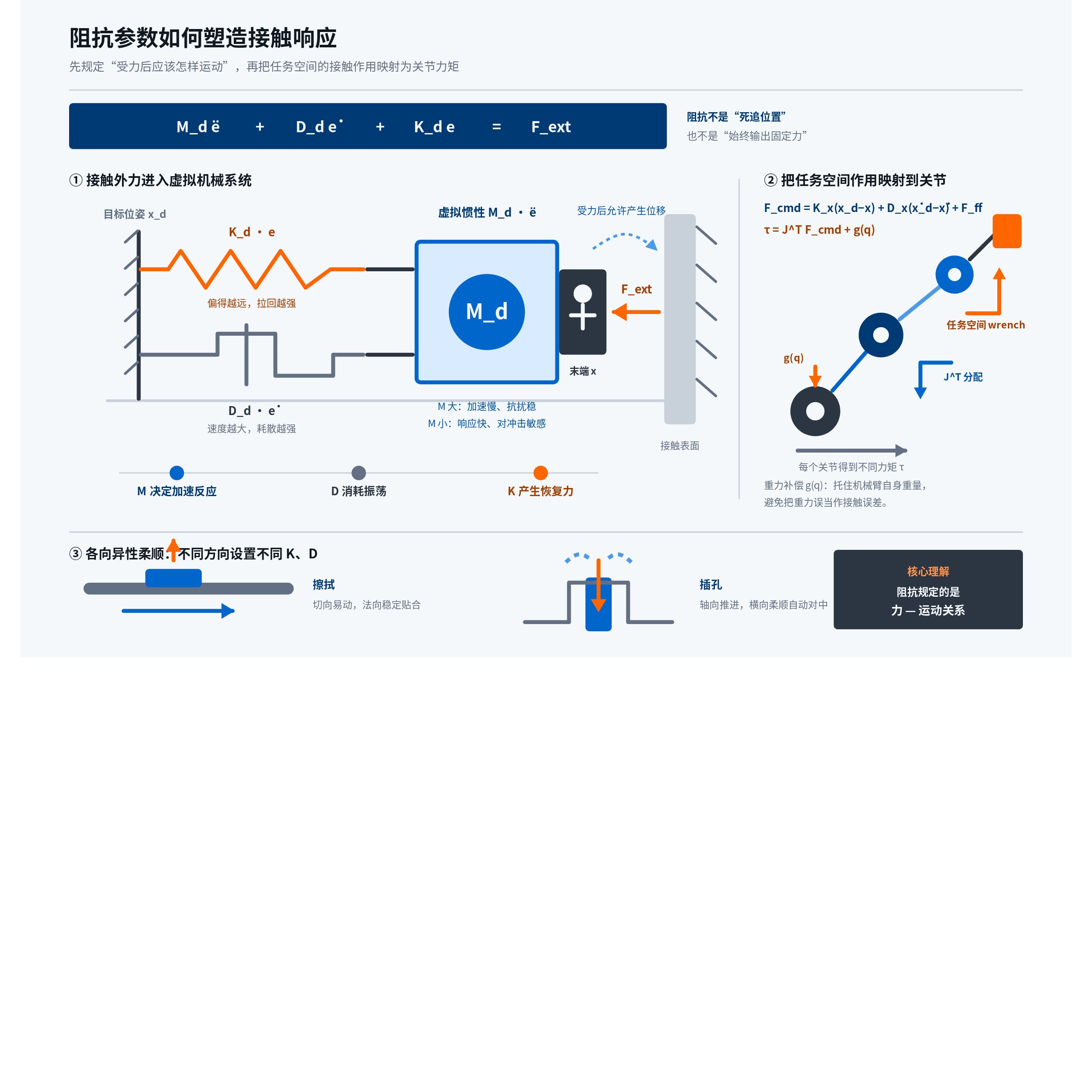
Here, the feedforward force represents known support forces, loads, or desired contact forces. Task-space stiffness and damping determine the robot’s compliance in each direction. During peg insertion, axial advancement can be limited while lateral compliance is maintained; during wiping, the robot can track a tangential trajectory while maintaining normal pressure.
5. Hybrid Position/Force Control
Use the selection matrix to specify the position-controlled subspace and to specify the force-controlled subspace:
Interpretation: Directions selected by the matrix S use position control, while the complementary subspace uses force control; the two are added to form the task-space command.
Derivation: If S is a projection matrix, S and I-S divide the task space into complementary directions. During wiping, for example, the tangential directions track a trajectory while the normal direction tracks pressure. S must be defined in a coordinate frame aligned with the contact geometry.
In words: “Some directions track position, while others track contact force.” The key issue is not the formula itself, but that the coordinate frame must be aligned with the contact geometry. If the surface normal is estimated incorrectly, the supposed normal-force controller will also push tangentially, causing slip.
6. What Tactile Sensing Actually Provides
| Signal | Directly Observable | Common Inferences |
|---|---|---|
| Six-axis force/torque | Resultant force and torque | Collision, load, contact direction |
| Fingertip array | Pressure distribution | Contact position, area, eccentricity |
| Vision-based tactile image | Surface-deformation texture | Slip, local geometry, shear |
| Motor current | Proxy for actuation force | Abnormal resistance and collision |
The advantages of tactile sensing are its high sampling rate and direct response to contact. Its limitations include locality, drift, latency, and differences between sensor domains. A policy can use tactile sensing to select the contact mode, while the low-level controller uses high-frequency force feedback to stabilize execution.
7. What Should a Learned Policy Output?
| Output Interface | What the Policy Learns | Primary Risk |
|---|---|---|
| End-effector pose | Geometric target | Contact force is generated indirectly by error |
| Desired force | Contact intensity | Contact frame and mode must be reliable |
| Impedance parameters | Stiffness, damping, equilibrium point | Parameter ranges may compromise stability |
| Skill or mode | Approach, search, insert, withdraw | Incorrect switching conditions |
Engineering systems commonly use a hierarchical interface in which “a low-frequency policy provides targets and modes, while a high-frequency controller ensures stability.” Having a neural network directly output torques is not impossible, but doing so pushes sampling, stability, safety, and hardware differences entirely into the data.
8. Minimal Visualization Experiment: One-Dimensional Contact
System model. Represent the end effector as a point mass and the wall as a unilateral Kelvin–Voigt element. Fix the control period at 1 ms and the policy or target update period at 50 ms so that the “low-frequency decision making, high-frequency control” interface can be observed independently.
Interpretation: The acceleration of the point mass is determined by the control force minus the environment reaction force. Compression occurs only after the mass moves beyond the wall position, and the environment reaction force is the sum of the compression-spring force and contact-damping force, constrained so that it cannot pull the object.
Derivation: First apply Newton’s second law: mass multiplied by acceleration equals the net force. Then use a nonnegative compression variable to represent unilateral contact. The Kelvin–Voigt model adds elastic and dissipative forces; the outer maximum excludes tensile forces from the ideal contact surface. Although this is not an exact material model, it is sufficient to expose the relationships among stiffness, damping, delay, and peak force.
| Experimental Dimension | Setting | Question to Answer |
|---|---|---|
| Controller | High-stiffness position control, low-stiffness position control, impedance control, normal-force control | Do performance differences arise from the target interface or the feedback structure? |
| Environment | Soft, medium, and hard wall stiffnesses; two contact-damping levels | Can the same control parameters remain stable across materials? |
| Timing | Feedback delays of 0, 10, and 30 ms; no jitter and random jitter | Is the stability margin eroded by delay? |
| Observation | No noise, force bias, timestamp misalignment, tactile frame drops | Is the controller using contact signals or chasing spurious signals? |
Logged quantities. For each run, save position, velocity, control force, environment force, and contact state. At minimum, report peak contact force, steady-state force error, 2% settling time, number of oscillations, maximum penetration, and the mechanical work injected by the controller in the contact direction.
Minimal ablation. On the same trajectory, sequentially mask tactile sensing, shuffle the temporal order of tactile observations, and add a fixed zero offset, while keeping vision and actions completely unchanged. If the policy genuinely uses tactile sensing, masking and permutation should produce distinct and interpretable degradation rather than merely random fluctuations.
Interpretation criteria. High position gains usually reduce free-space error but amplify peak force in a stiff environment. Insufficient damping manifests as multiple zero crossings and repeated bouncing after contact. As delay increases, the same parameter set may transition from decaying oscillation to divergent oscillation. If adding tactile sensing improves the average success rate while simultaneously worsening peak force and variance, the result cannot simply be interpreted as “tactile sensing is effective.”
9. Failure Modes
| Failure Mode | Observable Symptom | Root Cause | Validation and Remedy |
|---|---|---|---|
| Vision indicates “grasped,” but the object is still slipping | Tangential tactile signals continue to change while the grasp pose changes very little | Vision lacks local shear and microslip information | Perform tactile masking and permutation ablations; add slip classification or closed-loop grasp-force control |
| Zero drift is interpreted as persistent contact | A stable nonzero force remains under no load, and the contact threshold stays triggered | Sensor bias, thermal drift, or mounting preload | Calibrate under no load each episode; estimate bias online; use hysteresis for thresholds |
| Stable grasp in simulation, slip on the real robot | Tangential velocity is greater under the same normal force | Mismatch in friction, surface compliance, and the tactile domain | Test across materials; randomize friction and compliance; calibrate with real contact data |
| Impedance parameters exceed safe bounds | Peak force rises sharply, joints saturate, or high-frequency oscillation occurs after contact | The policy directly outputs unconstrained stiffness or damping | Limit parameter ranges and rates of change; project onto a positive-definite set; add force and power barriers |
| Tactile observations and actions are temporally misaligned | The model predicts “contact” before the action occurs, or applies correction in the opposite direction | Unsynchronized clocks, buffering delay, or resampling errors | Record hardware timestamps; perform a delay sweep; realign using causal windows |
| High success rate but unsafe contact | The task is completed, but peak force, impulse, or material damage exceeds limits | The reward and evaluation consider only the terminal state | Report success, peak force, impulse, energy, and safety-violation rate together |
10. Exercises
- Derive the equivalent stiffness when the robot spring and environment spring are connected in series.
- Define a hybrid-control coordinate frame with tangential position control and normal-force control for a table-wiping task.
- Explain why tactile sensing is valuable for slip detection but cannot replace global vision.
- Design a sensor-permutation experiment to verify that “the policy genuinely uses tactile sensing.”
- Define stability and safety constraints for learned impedance parameters.
Relationship to Other Tracks
Track A generates actions or impedance targets; Track B can predict contact outcomes; Track C can define value using success, peak force, and damage; Track D manages modes such as approach, contact, and recovery; and Track G handles synchronization, thresholds, monitoring, and regression testing.
11. Paper Evidence Matrix
The table below separates “what the paper reports,” “how the authors explain the mechanism,” and “the instructional conclusion drawn by this course,” avoiding the misrepresentation of course-level synthesis as the papers’ original wording.
| Work | Reported Evidence | Authors’ Explanation | Course Conclusion |
|---|---|---|---|
| Operational Space Control | Khatib formulated task-coordinate dynamics and force control in operational space and developed a unified representation of motion and force. | The author treats end-effector task variables as the natural space for control design, rather than first tracking in joint space and obtaining end-effector behavior indirectly. | If a VLA outputs end-effector targets or forces, it still requires an explicit task-space dynamics interface that maps them to joint torques. |
| Hybrid Position/Force Control | Raibert and Craig divided task coordinates into position-controlled and force-controlled directions for constrained manipulation. | The authors emphasize that control directions must be consistent with the task and contact constraints. | A selection matrix is not a fixed template; an incorrect surface-normal estimate turns “normal-force control” into simultaneous pushing and slipping. |
| Vision and Touch for Grasping | Calandra et al. jointly used vision and tactile sensing in grasping and regrasping experiments and compared different sensing combinations. | The authors treat tactile sensing as a signal that reduces visual uncertainty after contact, particularly for assessing grasp outcomes and triggering regrasping. | “Multimodality” demonstrates that a policy genuinely uses tactile sensing only when sensor ablation, permutation, and timing tests produce degradation consistent with the proposed mechanism. |
| Residual Reinforcement Learning | Johannink et al. trained a learned policy to produce residuals on top of an existing controller and validated the approach on real-robot contact tasks. | The authors use prior control structure to handle predictable components, allowing learning to focus on model error and contact effects that are difficult to model manually. | For contact-rich tasks, a policy need not relearn all torques; the learning objective can instead be a bounded correction to a stable controller. |
12. Cross-Reading
Read F1 first. Feedback, stability, and sampling delay determine whether the controllers in this lesson can operate safely in closed loop. Without the stability vocabulary from F1, it is easy to mistake “compliance” for simply reducing gains.
Then connect to Track A. A VLA can output poses, forces, impedance parameters, or contact skills. Different output interfaces change both the problem the policy actually learns and the stability responsibilities it assumes.
Then connect to Tracks B and C. A world model can predict contact outcomes, while value learning can jointly include success, peak force, damage, and recovery cost in the objective. However, prediction errors and omitted reward terms both translate into real contact risk.
Finally, connect to F3 and Track G. Friction, delay, sensor bias, and material compliance are all system-identification and Sim-to-Real issues. After deployment, they must be continuously validated through time synchronization, threshold monitoring, regression tasks, and safety-violation rates.