Original Feishu Document · Source Revision 13

💡

Course Overview: A successful demonstration is not the same as a reliable system. This lesson organizes data schemas, time synchronization, training reproducibility, statistical evaluation, failure classification, safety, deployment monitoring, and data feedback into a complete chain of evidence, answering whether an algorithmic improvement is real, reproducible, and deployable.

Learning Objectives

After completing this lesson, you should be able to define trainable and auditable data schemas; verify temporal alignment between observations and actions; design holdouts for tasks, objects, environments, and dynamics; quantify uncertainty in success rates; distinguish aggregate metrics from failure distributions; evaluate the calibration of value estimates or success probabilities; and establish a closed loop spanning deployment, monitoring, human intervention, data feedback, and retraining.

1. The Physical AI Chain of Evidence

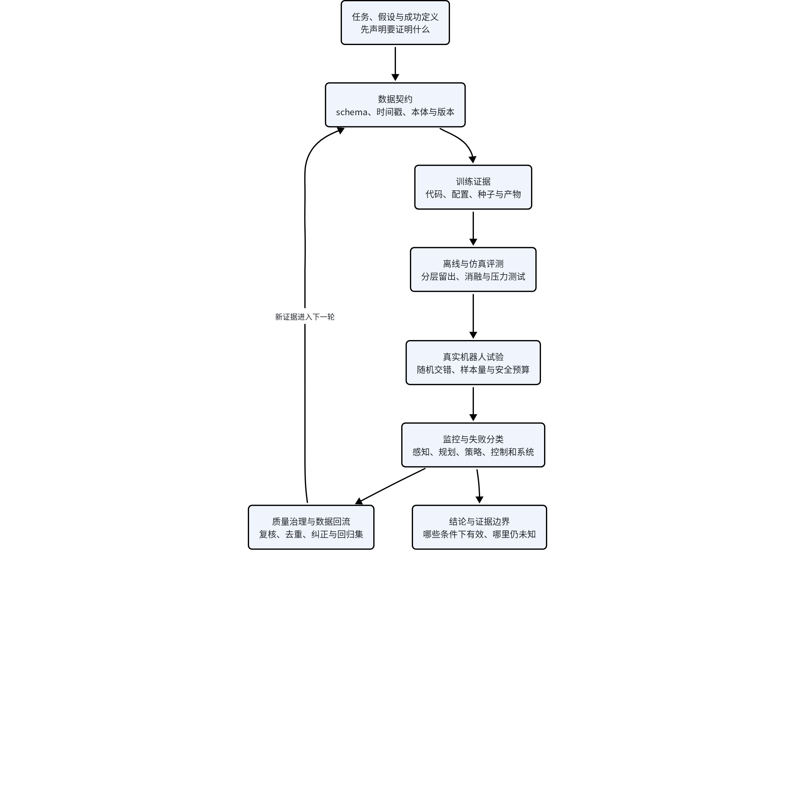
Every link in the chain must be traceable. If the data version, control frequency, or number of real-world trials is missing, then even complete model code cannot reveal whether an improvement came from the algorithm, data, hardware, or a change in the test protocol.

2. The Data Schema Is Part of the Algorithm

A robot episode requires at least the following:

Category	Fields	Why They Must Be Recorded
Observations	Images, depth, force sensing, proprioceptive state	Define the information actually available to the model
Actions	Command values, units, coordinate frames, frequency	Prevent semantic inconsistencies across data sources
Timing	Sensor, inference, transmission, and execution timestamps	Identify latency and causal misalignment
Task	Language goal, objects, initial conditions	Support task stratification and holdouts
Outcome	Success, stage, failure cause, intervention	Support value learning and evaluation
Embodiment	Robot, cameras, controller, calibration	Support cross-embodiment alignment and regression diagnosis
Versions	Data-collection code, model, configuration, hardware version	Support reproducibility and issue tracking

Equal image and action sequence lengths do not imply temporal alignment. Camera exposure, network transmission, model inference, and actuator response may cause to actually correspond to an earlier physical state.

3. Time Synchronization and Causal Alignment

Total latency can be decomposed as:

Interpretation: The total latency from the occurrence of a physical event until an action actually takes effect is the sum of sensing, transmission, model inference, and actuator response latencies.

Derivation: For the same sample, record the entry and exit times of every causal stage. When the durations of adjacent stages are summed, the intermediate time points cancel, leaving only the final execution time minus the initial acquisition time. Queue jitter and parallel pipelines change the per-sample latency distribution, so recording only the mean is insufficient.

Training samples should be constructed according to when an action actually takes effect, rather than paired simply by array index. A latency sweep can be used to find the offset that maximizes the correlation between actions and state changes, but the correlation peak does not necessarily equal the true causal latency and must be validated against hardware timestamps.

It is recommended to save all of the following:

• Observation acquisition time.
• Model inference start and end times.
• Action transmission time.
• Controller receipt and execution times.
• Time of the next observable physical response.

4. Training Reproducibility Requires a Complete Experimental Contract

Must Be Fixed or Recorded	Examples
Data manifest	Episode IDs, filtering rules, training/validation split
Model configuration	Backbone, action head, history length, Action Chunk
Optimization configuration	Learning rate, batch size, number of update steps, freezing, and gradient paths
Randomness	Seeds, sampler, augmentation, and initialization
Inference configuration	Number of sampling steps, temperature, replanning frequency
System versions	Code commit, dependencies, drivers, and firmware

Saving only the final checkpoint is insufficient for reproducibility. Data ordering, normalization statistics, tokenizer versions, and action adapters can also change the results.

5. A Success Rate Is Not an Error-Free Number

Given independent trials with successes, the estimated success rate is:

Interpretation: The empirical success rate equals the number of successful independent trials divided by the total number of trials.

Derivation: Encode each success as one and each failure as zero. The sample mean is then k divided by n. Under the independent and identically distributed Bernoulli assumption, this is also the maximum-likelihood estimate of the success probability. If trials are correlated or the success probability varies across conditions, this single mean conceals the stratified structure.

The approximate standard error is:

Interpretation: The approximate standard error of the empirical success rate equals the square root of the estimated success rate times the failure rate divided by the sample size.

Derivation: The variance of an independent Bernoulli variable is p times one minus p, and the variance of the mean of n independent samples is divided by n. Because the true p is unknown, substituting p_hat yields a plug-in estimate. When the sample is small or the success rate is close to zero or one, the normal approximation becomes inaccurate.

When the sample size is small or the success rate is close to 0 or 1, the normal approximation is unreliable; use a Wilson interval or a Beta-Binomial posterior instead.

5.1 Wilson Interval

For corresponding to the confidence level, the Wilson center is:

Interpretation: The center of the Wilson interval is the empirical success rate with a finite-sample correction, divided by the corresponding normalization factor.

Derivation: The Wilson interval is obtained by inverting the score test for a binomial proportion. Squaring the standardized inequality in the unknown p and rearranging it into a quadratic inequality yields two roots whose midpoint is this center. The correction pulls the extreme cases of zero successes or all successes moderately toward the interior, making it more stable than the direct normal interval.

The interval radius is:

Interpretation: The half-width of the Wilson interval is jointly determined by the confidence-level value z, the sample-proportion variance, and the finite-sample correction.

Derivation: Continuing to solve the quadratic inequality obtained from the score test, h is half the difference between the two roots. The final interval runs from the center minus h to the center plus h. As the sample size increases, the correction terms decay and the interval gradually approaches the common normal approximation.

Reporting “8/10 successes” is different from reporting “80%”: the former exposes the sample size and uncertainty.

6. Trials Are Not Necessarily Independent

Repeated trials conducted on the same day, with the same object and the same initial pose, are highly correlated. Treating them as independent samples underestimates variance. Results should be stratified by task, object, environment, robot, or data-collection batch, and analyzed using a stratified bootstrap or mixed-effects model.

Stratified reporting should include at least:

• Each task and task stage.
• Object category and specific instance.
• Difficulty of initial conditions.
• Environment and background.
• Robot embodiment and controller.
• Trial date and hardware status.

7. Training, Validation, and Genuine Generalization Holdouts

Holdout	What It Tests	Common Leakage
Object instance	Novel objects from known categories	The same object against different backgrounds
Task composition	Novel combinations of previously seen skills	Language paraphrases with identical actions
Environment structure	Novel spatial relationships	The same layout with different textures
Embodiment	Cross-robot transfer	Target-robot data included in pretraining
Dynamics	Changes in mass, friction, and compliance	Changing only appearance without changing physics
Failure states	Closed-loop recovery	Evaluating only expert initial states

“Open world” cannot be demonstrated using only photos of novel objects. It must be made explicit which task structures, physical parameters, and control conditions were excluded from training.

8. Failure Classification Matters More Than Average Success Rate

Failure Layer	Examples	Evidence to Inspect
Perception	Object-recognition or state-estimation error	Occlusion, viewpoint, confidence
Planning	Incorrect subgoal or ordering	High-level decision logs
Policy	Incorrect action pattern	Conditional action distributions and demonstration coverage
Control	Correct command but failed tracking	Target versus actual trajectories, forces, and saturation
System	Latency, dropped frames, process failures	Timestamps and runtime logs
Safety	Collisions, force spikes, emergency stops	Safety monitoring and intervention records
Evaluation	Inconsistent success judgments	Annotation protocol and review

The same whole-task failure rate can result from entirely different algorithmic bottlenecks. Without failure classification, additional data collection and model changes lack direction.

9. Calibration: Does the Model Know What It Does Not Know?

If a model predicts a success probability of , reliability requires that approximately 80% of samples assigned a prediction of 0.8 actually succeed. Expected Calibration Error can be written as:

Interpretation: Expected Calibration Error bins predictions by confidence, computes the absolute difference between the actual success rate and mean confidence in each bin, and then takes a weighted sum based on each bin’s fraction of the samples.

Derivation: Ideal calibration requires that approximately a fraction q of samples with predicted confidence q succeed. With finite data, the conditional probability cannot be estimated at every continuous value of q. Predictions are therefore first divided into B bins, with within-bin accuracy approximating the actual frequency and within-bin mean confidence approximating the predicted probability. Their differences are then empirically weighted. The result depends on the binning scheme and sample size and cannot be interpreted in isolation from the reliability diagram.

Low ECE is important for safety gating, human intervention, and candidate-policy selection. However, because ECE depends on binning, reliability diagrams and out-of-distribution detection results should also be presented.

10. Online Monitoring and Safety

A deployed system should monitor at least:

• Observation latency, inference latency, and control period.
• Action range, velocity, acceleration, and torque saturation.
• Contact forces, collisions, and slipping.
• Model uncertainty or success probability.
• Task stage and completion detection.
• Human intervention, emergency stops, and recovery.

The safety system should be independent of the learned policy. The policy may propose actions, while a deterministic safety layer enforces speed limits, workspace constraints, collision constraints, and force thresholds.

11. Data Feedback Does Not Mean Retraining on Every Failure

Deployment data should pass through the following process:

1. Automatically detect anomalies and failures.
2. Classify them by failure layer.
3. Extract the critical time windows.
4. Add labels for success, stage, contact, and human corrections.
5. Deduplicate and balance tasks and difficulty levels.
6. Add the data to dedicated training or evaluation sets.
7. Redeploy only after regression testing.

Incorrect labels, system failures, and policy failures must not be mixed into a single “failure data” bucket; otherwise, the model will learn incorrect causal relationships.

12. OpenPI’s Role in the Systems Roadmap

OpenPI provides models, data adaptation, and training infrastructure, but a complete system also requires:

OpenPI Can Provide	The Team Must Still Build
Model implementations and checkpoints	Task definitions and real-robot safety
Data formats and conversion	Time synchronization, quality labels, and version governance
Training and inference code	Evaluation protocols, monitoring, rollback, and data feedback
Baseline configurations	Target-embodiment adaptation and system validation

Getting the framework to run proves only that the software pipeline works; it does not prove that the data is correct, the algorithm is effective, or the robot is reliable.

13. Minimum Trustworthy Experiment

For a new policy modification, the minimum evidence should include:

Comparison targets. Select one deployed baseline and one candidate new policy. Freeze the data version, task definitions, controller, hardware, success criteria, and safety thresholds. Both the old and new models must execute exactly the same preregistered protocol.

Evidence Layer	Minimum Setup	Must Be Answered Before Release
Training reproducibility	At least three independent training runs; save data manifests, configurations, code, dependencies, and random seeds	Does the improvement exceed training variance?
Holdout design	Stratified holdouts for tasks, object instances, environment structures, dynamics, and failure initial states	Was the test set genuinely excluded from training and hyperparameter tuning?
Real-world trials	Run the old and new models in stratified, randomized, interleaved order across conditions, recording complete hardware timestamps	Did date, temperature, wear, or operator become confounding factors?
System ablations	Shift action alignment by several frames in each direction; inject latency, dropped frames, and reduced controller frequency	Does the model improvement depend on an incidental timing or system configuration?
Statistical reporting	Number of successes/total trials, Wilson intervals, stratified bootstrap, failure distribution, and ECE	Is the average improvement accompanied by degradation in tail performance or calibration?
Safety gates	Peak force, impulse, saturation, emergency stops, intervention rate, and recovery time	Does the candidate policy regress on any hard constraint?

Minimum deliverables. One plot comparing stratified success rates and confidence intervals for the old and new models; one stacked plot of failure types; one performance heatmap over latency and dynamics conditions; one reliability diagram; and one manifest tracing each model version to its data, code, hardware, and every real-world trial.

Release rule. Specify one primary task metric and all hard safety metrics in advance. Expansion to a broader staged rollout is permitted only when interval-based evidence for the primary metric supports an improvement and no safety metric exceeds its regression threshold. The primary metric must not be changed after reviewing the results.

14. Exercises

1. Design a complete schema for a robot episode, including timestamp and version fields.
2. Calculate the difference in uncertainty between success rates of 8/10 and 80/100.
3. Design a split that prevents leakage of objects and task structures.
4. Classify ten failure videos into perception, planning, policy, control, and system failures.
5. Plot a reliability diagram for a value model and explain ECE.
6. Design release gates for the “deployment → failure → data → retraining → regression testing” loop.

Papers and Engineering Lab

OpenPI Practice and ArcheBase Data Production

15. Evidence Matrix for Papers and Benchmarks

Dataset scale and benchmark scores constitute evidence only when the schema, splits, evaluation protocol, and real-system conditions are traceable.

Work	Facts from the Paper	Authors’ Interpretation	Course Assessment
Open X-Embodiment	This work aggregates multi-institution, multi-robot, and multi-task data and trains the cross-embodiment RT-X policy family.	The authors explore cross-robot knowledge transfer through a unified data format and large-scale heterogeneous mixtures.	A unified schema is part of the algorithmic capability; missing action semantics, coordinate frames, frequencies, or embodiment metadata can cause scale to create spurious commonality.
DROID	DROID collects large-scale real-world robot manipulation data across scenes and operators and provides a unified collection system.	The authors emphasize the importance of diverse real-world environments and standardized hardware data pipelines for general-purpose policies.	Beyond data volume, audits must cover scene correlations, operator bias, hardware versions, and train-test instance leakage.
RoboMimic	RoboMimic systematically compares multiple offline imitation-learning methods, data qualities, and task settings.	Using a unified benchmark, the authors reveal the sensitivity of algorithmic results to data sources, observations, and training details.	A “same-dataset comparison” still requires fixed preprocessing, normalization, action interfaces, and evaluation initial states; otherwise, it is not a controlled ablation.
LIBERO	LIBERO builds a continual robot-learning task suite with variations in objects, spatial relationships, goals, and long-horizon sequences.	The authors use structured task families to evaluate knowledge transfer and forgetting rather than only single-task success rates.	Generalization claims must specify whether the holdout concerns language expressions, object instances, spatial structures, or skill compositions.
Guo et al.｜Calibration	This work systematically evaluates the probability calibration of modern neural networks and compares methods such as temperature scaling.	The authors distinguish classification accuracy from confidence reliability, showing that highly accurate models can still be overconfident.	Before robot success probabilities are used for intervention and gating, they must be conditionally calibrated; global ECE must not conceal dangerous subgroups.

16. Cross-Reading

Read alongside all algorithmic roadmaps. Conclusions about VLAs, world models, value learning, hierarchical planning, and control all depend on the same data versions, holdouts, and real-world closed-loop protocols. Roadmap G is not ancillary engineering; it is the measurement system that determines whether the conclusions are valid.

Read alongside F3. Timestamps, actuator identification, and parameter versions affect both Sim-to-Real and the causal correctness of data labels.

Read alongside Roadmap E. Cross-embodiment joint training is auditable only when action interfaces and embodiment metadata are traceable; otherwise, the model may merely memorize data-source identities.

Read alongside G1–G4. This lesson presents the overall chain of evidence; subsequent lessons examine statistical uncertainty, data versioning, deployment monitoring, and OpenPI systems engineering in greater depth.