

Original Feishu Document · Source Revision 29
💡
Mechanisms lesson: “The success rate increased from 70% to 80%” is not a conclusion unless the experimental unit, sample size, task stratification, random seeds, confidence interval, cost of failure, and selection process are specified. This lesson reframes robot evaluation as a statistical inference problem.
Learning Objectives
After completing this lesson, you should be able to define independent experimental units; derive the Bernoulli success-rate estimate and its standard error; use Wilson intervals and the Beta-Binomial model; handle task stratification, repeated measurements, and multiple comparisons; and explain calibration, selective prediction, and risk-coverage curves.
1. Define the Random Variable First
Let the outcome of a single trial be:
Reading: The outcome of trial i is a Bernoulli random variable with success probability p, taking the value one for success and zero for failure.
Derivation: When a trial retains only two mutually exclusive outcomes—success or failure—its probability mass function is determined by a single parameter p. This model requires the trial distribution to be fixed in advance. If tasks, objects, and initial conditions vary across batches, p should be expressed as a conditional or hierarchical parameter rather than assumed to be a global constant.
The sample success rate is:
Reading: The empirical success rate is the sample mean of n binary trial outcomes.
Derivation: Because each Y_i equals one on success and zero on failure, their sum is exactly the number of successes k. The sample mean therefore equals k divided by n. Under the independent and identically distributed Bernoulli model, it is also the maximum-likelihood estimate of p.
This estimate applies only to a clearly defined trial distribution. If the tasks, objects, operators, and initial states change every day, a single global success rate mixes conditional differences into one parameter. Results should instead be reported by stratum or modeled conditionally.
2. Why 8/10 Is Weak Evidence
Under the independent and identically distributed assumption:
Reading: The variance of the empirical success rate for independent Bernoulli trials equals the success probability times the failure probability, divided by the sample size.
Derivation: The variance of a single Bernoulli variable is p times one minus p. Variances add when independent variables are summed, and the sample mean introduces division by n squared. The result is therefore n times the single-trial variance divided by n squared. When trials are correlated, covariance terms appear and the effective sample size is smaller than the nominal number of trials.
Substituting for gives the standard error. With small samples, the normal approximation is poor, especially when the success rate is close to 0 or 1. The center of the Wilson interval is:
Reading: The center of the Wilson interval is the empirical success rate with a finite-sample correction, divided by the corresponding normalization factor.
Derivation: Starting from the score test for a binomial proportion and solving the inequality that constrains the standardized error to be no greater than z in magnitude yields a quadratic inequality in the unknown p. The midpoint of its two roots is the expression above. It moderately shrinks extreme small-sample estimates toward the interior of the interval.
Its half-width is:
Reading: The half-width of the Wilson interval is jointly determined by the confidence level, the variance of the sample proportion, and the finite-sample correction.
Derivation: Continuing to solve the quadratic inequality from the score test, half the difference between the two roots is h. The confidence interval therefore extends from the center minus h to the center plus h. As n increases, the correction terms decay and the interval gradually approaches the familiar large-sample approximation.
The Wilson interval is more suitable than the Wald interval—which directly adds and subtracts 1.96 standard errors from the empirical proportion—for small samples and extreme success rates. It still relies on the assumption of independent trials, however; within-task correlations should be handled using a cluster bootstrap or a hierarchical model.
3. Bayesian Interpretation: Beta-Binomial
Assume a prior . After observing successes and failures:
Reading: After observing s successes and f failures, the posterior distribution of the success probability remains a Beta distribution, with the two shape parameters incremented by the success and failure counts, respectively.
Derivation: The likelihood of Bernoulli data is proportional to p raised to the power s times one minus p raised to the power f. The Beta prior is proportional to p raised to the power alpha minus one times one minus p raised to the power beta minus one. Multiplication adds the exponents directly, yielding the conjugate posterior.
The Beta-Binomial formulation makes it convenient to compute the posterior probability that one method has a higher success rate than another, but the prior, the exchangeability of trials, and the data-selection process must be transparent. When different tasks have different success rates, use a hierarchical Beta-Binomial model rather than directly adding all counts together.
4. Why Trials Are Not Independent
One hundred consecutive runs on the same robot in the same scene may share temperature, lighting, calibration, and wear conditions. The effective sample size is therefore less than 100. Date, robot, task, object, or operator should be treated as a cluster, with hierarchical bootstrap, mixed-effects models, or cluster-level aggregation used for analysis.
A simple hierarchical logistic model is:
Reading: For trial i in task or scene j, the log-odds of success are determined by the sum of the population-level intercept, the method effect, and the random difficulty offset for that task.
Derivation: For a binary outcome, the logistic link maps a linear predictor to a probability between zero and one. Representing unobserved task-level difficulty as a zero-mean random intercept allows trials within the same task to share correlation, while beta_1 estimates the average method difference across tasks.
The random effect represents the difficulty offset shared by a task or scene. It prevents “one method happened to be tested more often on easy tasks” from being mistaken for an algorithmic gain, and it can estimate heterogeneity across tasks. When the number of tasks is too small, however, the random-effect variance itself will be highly unstable.
💡
Interactive Validation|Wilson Interval, Calibration, and Risk-Coverage Lab
Vary the number of trials, success rate, and degree of calibration to observe Wilson interval width, miscalibration risk, and safety coverage.
Wilson Interval, Calibration, and Risk-Coverage Lab
:::5. Paired Experiments Are More Powerful Than Independent Comparisons
If methods A and B are tested under the same initial states, objects, and perturbations, the difference within each pair can be analyzed to remove noise due to scene difficulty. McNemar’s test can be used for binary outcomes, and a paired bootstrap can be used for continuous metrics. Pairing is valid only if test order, wear, and environmental memory do not systematically favor either method.
For the binary outcomes of A and B under the same test condition, consider only pairs in which the two methods disagree. Let n_01 denote cases in which A fails and B succeeds, and n_10 denote cases in which A succeeds and B fails:
Reading: The continuity-corrected McNemar statistic is the squared difference between the counts of the two types of discordant pairs, divided by the total number of discordant pairs.
Derivation: Under the null hypothesis, the two directions of disagreement should occur with equal probability. Conditional on the total number of discordant pairs, n_01 therefore follows a binomial distribution with success probability one-half. For large samples, this binomial deviation is standardized as a chi-squared statistic. When there are few discordant pairs, use the exact binomial test directly.
6. Do Not Report Significance Alone
| Must Be Reported | Question Answered |
|---|---|
| Effect size | How large is the practical improvement? |
| Confidence/credible interval | How wide is the uncertainty range? |
| Samples and stratification | Where does the evidence come from? |
| Cost of failure | Was the improvement achieved at the expense of collisions or human interventions? |
| Prespecified primary metric | Was the most favorable result selected from many metrics? |
7. Multiple Comparisons and Leaderboard Overfitting
Testing many checkpoints, prompts, random seeds, and task slices simultaneously and then reporting only the best result introduces selection bias. Separate the development set from the final locked test set, record all experiments, and control the family-wise error rate or false discovery rate when necessary. Most importantly, limit repeated access to the final test set.
8. Calibration: Does Confidence Correspond to the True Frequency?
If the model predicts a success probability of , ideal calibration satisfies:
Reading: If the model is well calibrated, then among all trials assigned a predicted confidence of q, approximately a fraction q should succeed in the long run.
Derivation: Calibration interprets probabilistic predictions as conditional frequencies: among samples with the same predicted value, the mean outcome should equal that value. With finite data, this condition can only be tested approximately through binning, smoothing, or calibration models.
Expected Calibration Error:
Reading: ECE takes the absolute difference between the observed success rate and mean confidence in each confidence bin, then computes a weighted sum using the proportion of samples in each bin.
Derivation: Ideal calibration requires equality of conditional frequencies over a continuous range of confidence values, but finite samples do not permit pointwise estimation. The range is therefore approximated piecewise using B bins. Accuracy within each bin estimates the outcome frequency, while mean confidence within the bin estimates the predicted probability. Their empirically weighted difference is the ECE.
ECE depends on the binning scheme and should not be used alone. The Brier score, negative log-likelihood, and reliability diagram should also be examined.
Brier score. In addition to calibration, the squared error between the probabilistic prediction and the true outcome should also be penalized:
Reading: The Brier score is the mean squared difference between the predicted probability of success and the actual binary outcome for each trial.
Derivation: Viewing the probabilistic prediction as an estimate of the mean of a Bernoulli outcome, squared error achieves its minimum expected value at the true conditional probability. It is therefore a proper scoring rule. It reflects both calibration and discrimination, and lower values are better, but it should still be reported by task difficulty and safety-critical subgroup.
9. Selective Prediction and Risk-Coverage
A robot can request human assistance, perceive again, or adopt a conservative policy when confidence is low. Let the acceptance threshold be :
Reading: Coverage at threshold tau is the proportion of trials for which model confidence reaches the threshold and autonomous execution is permitted.
Derivation: A selective system accepts only samples whose confidence is at least tau, so the acceptance event is c greater than or equal to tau. Its probability can be estimated by the proportion of samples in the test set that satisfy this condition. As tau increases, coverage generally decreases.
Reading: Selective risk at threshold tau is the conditional probability of failure among all trials permitted to execute autonomously.
Derivation: First use c greater than or equal to tau to select the acceptance set, then compute the mean failure rate within that set. As the threshold increases, the system abstains on more low-confidence trials and risk generally decreases. If confidence is miscalibrated or distribution shift is present, however, risk may not improve monotonically.
A risk-coverage curve can answer: “To reduce the failure rate to 2%, what fraction of autonomous executions must be relinquished?” This is more directly relevant to deployment decisions than a single AUROC value.
Formula Visualization|How Confidence Thresholds Change Risk and Coverage

10. Minimal Visualization Experiment
Generate data. Construct 20 tasks of varying difficulty. Each task includes shared random difficulty, a date-level batch effect, and several paired initial conditions. Policies A and B are executed in randomized interleaved order under the same conditions, and a confidence score with systematic bias relative to the true success probability is generated.
| Experimental Module | Comparison | Expected Lesson |
|---|---|---|
| Sample size | Wilson intervals for 8/10, 16/20, 80/100, and 160/200 | The same proportion does not imply the same strength of evidence |
| Correlation | Naive pooling, episode-level bootstrap, and task- or date-level cluster bootstrap | How treating correlated trials as independent samples underestimates interval width |
| Paired design | Independent difference in proportions, paired bootstrap, and McNemar’s exact test | How statistical power changes after shared difficulty is removed |
| Hierarchical effects | Micro-average, macro-average, hierarchical logistic model, and per-task effects | Whether the aggregate improvement comes from changing the weight of easy tasks |
| Calibration | Reliability diagram, ECE, Brier score, and results before and after temperature scaling | Whether high accuracy is accompanied by overconfidence |
| Selection bias | Repeatedly select the best of 20 checkpoints, then verify it on a locked test set | How leaderboards and repeated test-set access create optimistic bias |
Minimal output. Success-rate plots with intervals, a plot of paired per-task differences, the cluster-bootstrap distribution, a reliability diagram, a risk-coverage curve, and a scatter plot of “best development-set value versus locked test-set value.”
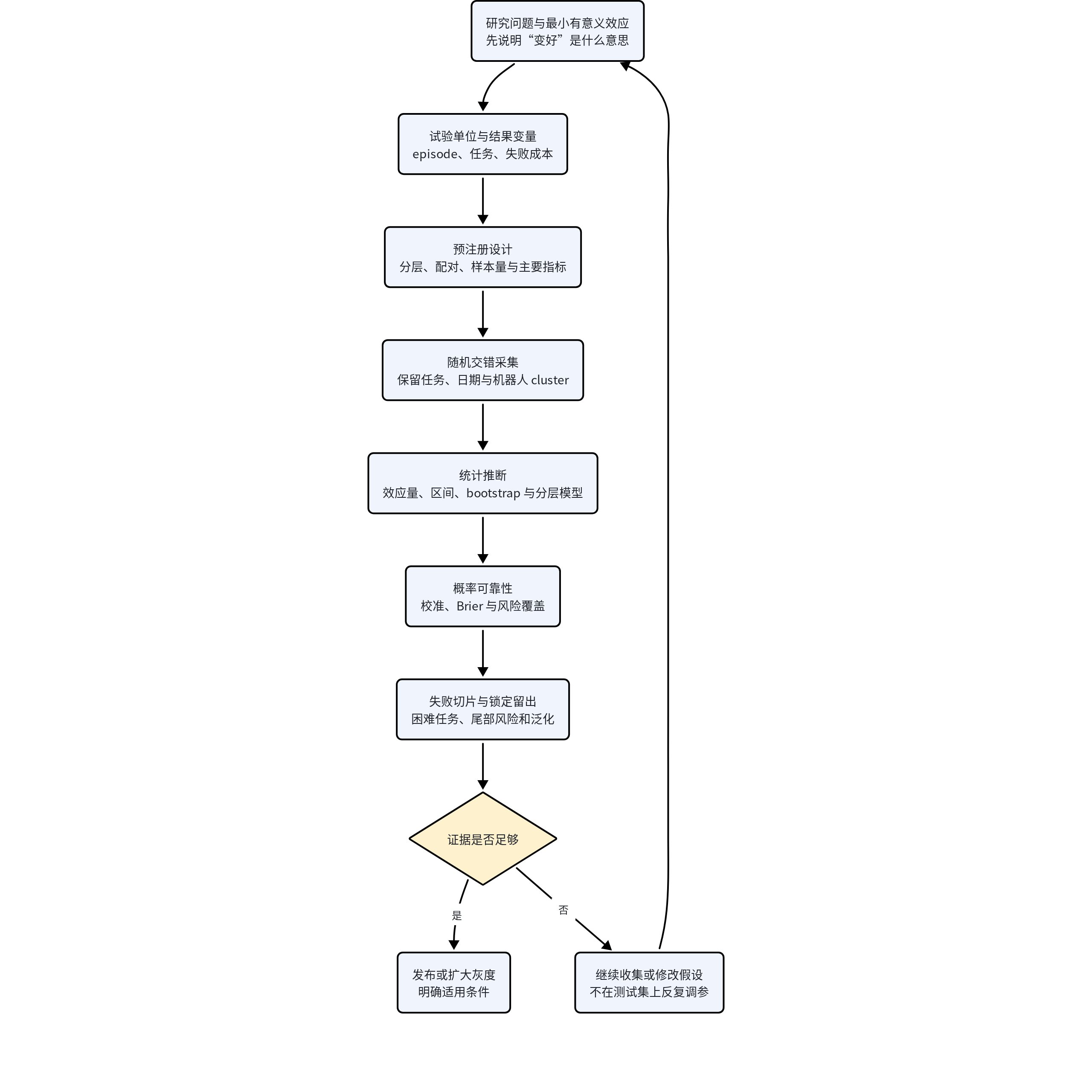
Release criteria. Preregister the primary effect, stratification units, and safety metrics; report all training repetitions and test conditions. Claim that the system is “better overall” only when the interval for the primary effect, difficult-task slices, and safety risk all support improvement.
11. Common Failure Modes
| Failure Mode | Why It Is Wrong | Decisive Check | Remedy |
|---|---|---|---|
| Treating frames as the sample size | Frames within the same episode are highly correlated and cannot be counted repeatedly as evidence of success | Compare intervals from frame-level and episode-level bootstraps | Use the episode or a higher-level cluster as the resampling unit |
| Micro-averaging obscures difficult tasks | A larger number of trials on easy tasks will dominate the aggregate success rate | Plot the macro-average, per-task effects, and task weights together | Fix sampling quotas in advance and report stratified results |
| Repeatedly tuning on the test set | The selection process fits test noise and presents it as model improvement | Compare the best development-set result with a one-time evaluation on the locked test set | Restrict test-set access and record all experiments |
| Changing the success definition after the experiment | Allowing outcomes to determine the labeling rules introduces researcher degrees of freedom | Audit raw videos, annotation versions, and modification timestamps | Preregister success criteria and conduct blinded review of disputed samples |
| Reporting only the mean | Heterogeneous tasks and high-cost failures are averaged away | Examine confidence intervals, quantiles, failure types, and safety costs | Report the effect distribution and tail risk |
| Treating language confidence directly as success probability | Token probabilities are not calibrated for physical-task outcomes | Reliability diagram, Brier score, ECE, and distribution-shift slices | Calibrate against real-robot outcomes and establish risk-coverage gates |
12. Exercises
- Compute and compare the Wilson intervals for 16/20 and 160/200.
- Design a paired experiment stratified by object, initial pose, and date.
- Explain why a cluster bootstrap should resample by episode or date.
- Construct an example of Simpson’s paradox in which the aggregate success rate improves while performance degrades on every difficult task.
- Define a risk-coverage release threshold for “request human assistance when confidence is low.”
Relationship to Other Tracks
Every track must ultimately withstand the statistical scrutiny introduced in this lesson. The generalization claims in Track A, predictive gains in B, empirical improvements in C, long-horizon tasks in D, cross-embodiment transfer in E, and contact safety in F cannot be demonstrated using only a single mean success rate.
13. Evidence Matrix for Statistical Methods and Evaluation Papers
| Work | Facts from the Paper | Authors’ Interpretation | Course Assessment |
|---|---|---|---|
| Wilson 1927|Binomial Interval | Wilson derived an interval for a binomial proportion through the score test, avoiding the anomalous behavior of the simple Wald interval with small samples and near the boundaries. | The author constructed the interval from the estimating equation rather than by directly adding and subtracting standard errors from the empirical proportion. | Robot experiments usually have few trials. Report Wilson or more robust intervals by default rather than percentages alone. |
| Efron 1979|Bootstrap | The bootstrap uses resampling from the empirical distribution to approximate the sampling distribution of a statistic. | The author replaced the unknown population distribution with the empirical distribution of the observed data and estimated uncertainty through repeated resampling. | The resampling unit must match the independence structure; bootstrapping by frame creates a spurious sample size. |
| Bates et al.|lme4 | This work systematically describes the software implementation and estimation methods for linear and generalized linear mixed-effects models. | The authors use fixed effects to represent population-level relationships and random effects to represent between-group heterogeneity and within-group correlation. | Experiments spanning tasks, dates, and robots should model clusters explicitly rather than flattening all episodes into one pool. |
| Benjamini & Hochberg 1995|FDR | This method controls the expected proportion of false discoveries in multiple hypothesis testing. | The authors distinguish per-comparison error rates from the proportion of errors in the set of discoveries and provide a more powerful procedure than Bonferroni correction. | When there are many checkpoints, task slices, and metrics, lock the primary analysis first. FDR cannot correct for repeated access to the final test set. |
| Guo et al. 2017|Calibration | This work shows that modern neural networks can be accurate yet overconfident and compares calibration methods such as temperature scaling. | The authors evaluate classification correctness separately from probabilistic reliability. | Robot gating requires calibration of physical-task success probabilities, not language-model token probabilities. |
| Geifman & El-Yaniv|Selective Classification | This line of work studies the tradeoff between risk and coverage when a model is allowed to reject some samples. | The authors use confidence ranking to select a more reliable subset and analyze how reduced coverage lowers error risk. | Physical AI systems should report risk-coverage curves, placing “how often human assistance is requested” and “how often autonomous execution fails” on the same plot. |
14. Cross-Reading
Read alongside G0. G0 defines the chain of evidence; G1 provides statistical tools for success rates, correlation, calibration, and selective deployment.
Read alongside all algorithm tracks. Claims of generalization, value improvement, planning gains, and control robustness must specify the independent experimental unit, effect size, interval, and failure distribution.
Read alongside G3. Risk-coverage curves and calibration determine when the online system should execute autonomously, degrade gracefully, or request human assistance.